
5 Steps to Quantify Betting Edge with Monte Carlo
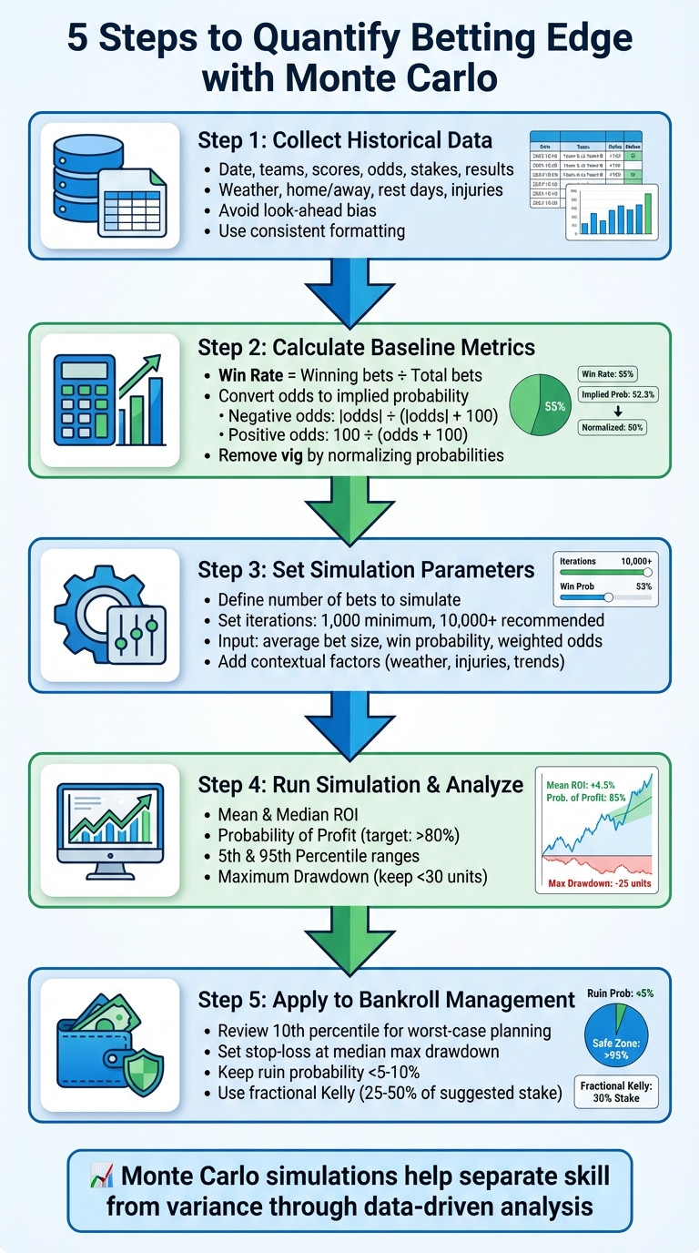
Monte Carlo simulations are a powerful way to evaluate your betting edge, helping you make smarter decisions based on data rather than guesswork. By simulating thousands of betting scenarios, you can identify your long-term profit potential, understand the role of variance, and optimize your bankroll management. This guide breaks the process into five clear steps:
- Gather Historical Data: Collect detailed records of your past bets, including odds, stakes, results, and contextual factors like weather or injuries.
- Calculate Key Metrics: Determine your win rate, implied probabilities, and adjust for the sportsbook’s vig.
- Set Simulation Parameters: Define the number of bets, iterations, and variables like average bet size and win probability.
- Run Simulations: Use tools like Excel or Python to simulate thousands of betting outcomes, analyze ROI, profit probability, and risk metrics.
- Apply Insights: Use results to refine your staking strategy, prepare for losing streaks, and manage risk effectively.
Monte Carlo simulations offer a practical approach to evaluate betting strategies, helping you separate actual skill from random variance. Whether you’re using basic tools like Excel or advanced platforms, this method equips you with the insights needed to make data-driven decisions and protect your bankroll.
5 Steps to Quantify Betting Edge Using Monte Carlo Simulations
Monte Carlo Simulation Tutorial: How Variance Impacts Your Betting Results
Step 1: Collect and Organize Your Historical Betting Data
Accurate simulations rely on solid, reliable data. The outcomes of Monte Carlo simulations are only as good as the information you feed into them. As EdgeSlip notes:
The quality of your data dictates the ceiling of your model.
If your records are incomplete or inconsistent, even the most advanced simulation will produce misleading results.
Identify the Key Data Points You Need
Start by compiling a complete betting history. At a minimum, include these details: the date, teams, final score, American odds (convert them using the formula: for positive odds, 100/(odds+100); for negative odds, |odds|/(|odds|+100)), stake, and result. These basics ensure your simulations are grounded in accurate probabilities.
Beyond the basic outcomes, consider adding situational variables that could influence game results. Examples include:
- Weather conditions (especially for outdoor sports)
- Home vs. away settings
- Rest days between games
- Travel distances
- Injury reports, particularly for key players like quarterbacks
Advanced metrics, such as Expected Points Added (EPA), yards per play, and offensive/defensive efficiency ratings, can also provide deeper insights for your analysis.
One crucial principle: avoid look-ahead bias. Only include data that was available before the game began. For instance, if you're evaluating a bet placed on 09/15/2024, don't use statistics from games played after that date.
Organize Your Data for Analysis
Consistency is key when structuring your data. Use a format where each row represents a single bet, and each column corresponds to a specific variable - like date, home team, away team, final score, odds, stake, and result.
To keep things tidy:
- Use consistent team names (e.g., avoid mixing "KC" with "Kansas City Chiefs").
- Format all dates uniformly (MM/DD/YYYY).
- Ensure column headers are clear and standardized.
If you're working with multiple bet types or leagues, it might help to use separate sheets or tabs. Just make sure every dataset follows the same column structure. A well-organized dataset is essential for calculating accurate metrics in the next phase.
Step 2: Calculate Your Baseline Metrics and Win Probability
After organizing your data, the next step is to compute the key metrics that will drive your Monte Carlo simulation. These foundational numbers - your win rate and average odds - are crucial for generating accurate projections.
Calculate Win Rates and Average Odds
To find your win rate, use this formula: win rate = (winning bets / total bets). For example, if you’ve placed 200 bets and won 110, your win rate would be 55%.
Next, convert American odds into implied probabilities. Here’s how:
- For negative odds: |odds| / (|odds| + 100)
- For positive odds: 100 / (odds + 100)
For instance, a bet at -150 has an implied probability of 150 / (150 + 100) = 60%, while a bet at +200 translates to 100 / (200 + 100) ≈ 33.3%.
To remove the vig (or sportsbook edge), normalize the implied probabilities by dividing each by the market total. In a standard -110/-110 market, the total implied probabilities often add up to 104.8%, reflecting a 4.8% hold by the sportsbook. Dividing each implied probability by 1.048 adjusts them to a fair 100% total.
As betting analyst Joseph Buchdahl explains:
"The larger my betting history, the more probable it is that the actual performance will be closer to expectation."
A larger sample size makes your baseline metrics more dependable. With enough data, Monte Carlo simulations can better determine whether past profits result from actual skill or random variance. For example, simulations based on 1,521 bets with a 4.04% theoretical edge revealed that bad luck could still lead to losses in about 17% of scenarios.
Once these metrics are established, you can refine them further by accounting for external influences.
Adjust for Contextual Factors
Fine-tune your win rates by considering elements like weather conditions, home-field advantage, rest periods, and injuries. Use advanced stats such as EPA (Expected Points Added), success rate, and efficiency ratings to enhance your team evaluations.
Pay attention to performance differences under varying conditions. For example, if your win rate is 58% on home underdogs but drops to 48% for road favorites, segmenting your data can help pinpoint where your edge lies.
These refined probabilities will serve as the foundation for configuring your Monte Carlo simulation inputs.
Step 3: Set Up Your Monte Carlo Simulation Parameters
Now that you’ve established your baseline metrics, it’s time to configure your simulation. This step involves deciding how many scenarios to test and identifying the variables that will influence each outcome. Properly setting these parameters is crucial for generating reliable results.
Define Your Simulation Scope and Variables
Begin by determining how many bets you want to simulate. This could be a fixed number, like 500 wagers, or it could span a specific timeframe, such as an entire NFL season. Next, decide on your iteration count - the number of times the simulation will replay the sequence of bets. For most bettors, running at least 1,000 iterations is a good starting point, but 10,000 or more iterations are often recommended to capture less common outcomes. Betting analyst Miguel Figueres emphasizes this point:
"The higher the number of simulations, the more precise results we are obtaining".
For example, in November 2018, Joseph Buchdahl conducted a Monte Carlo simulation on 1,521 bets with a 4.04% expected value. Using 100,000 iterations in Excel, he discovered that even with a 4% edge, a loss occurred in 17% of the simulated scenarios. The outcomes ranged from a -12.23% yield to a 23.26% yield. This highlights how higher iteration counts provide a clearer picture of potential variance.
You’ll also need to input key variables like your average bet size (e.g., 2% of your bankroll), win probability (derived from vig-free odds), and average weighted odds. These factors fuel the random sampling process that determines whether each bet in the simulation wins or loses.
Once these basics are in place, you can add layers of complexity to reflect real-world conditions.
Add External Factors to Your Simulation
To make your simulation more realistic, incorporate situational variables that influence actual outcomes. These might include team performance trends, injuries, weather conditions, rest days, or home-field advantage. For example, using rolling averages from recent games instead of season-long stats can help your model account for momentum shifts or changes in form.
In September 2025, professional handicapper MG used ChatGPT to simulate 10,000 NFL seasons for a top-down model. Each season included 67 plays, with win rates sampled from historical averages (58%, 60%, and 44%) and standard -110 odds. The simulation revealed a 53.2% probability of profit and a 95th percentile upside of +25.2 units. By factoring in these contextual elements, the simulation offered a more nuanced view of potential variance.
Step 4: Run the Simulation and Analyze the Results
Once your simulation parameters are set, it’s time to run the simulation and see how your strategy performs. This step involves using a Monte Carlo simulation to generate random values for each bet, comparing them against your win probability, and then summing the outcomes over thousands of iterations. For each bet, the simulation generates a random number between 0 and 1. If the number falls below your win probability, the bet is a win; otherwise, it’s a loss. By repeating this process thousands of times, you’ll create a distribution of potential outcomes.
Focus on These Key Output Metrics
When analyzing the results, there are a few critical metrics to watch:
- Mean and Median ROI: The mean represents your average expected return, while the median reflects the typical outcome you’re likely to experience. A median above zero indicates a strategy with positive expectancy.
- Probability of Profit: This shows the percentage of simulations that ended with a net gain. For long-term strategies, aim for a probability of profit above 80%.
- Percentile Ranges: The 5th percentile represents your worst-case scenario (only 5% of runs perform worse), while the 95th percentile represents your best-case scenario (only 5% of runs perform better). These percentiles give you a realistic range of outcomes.
- Maximum Drawdown: This measures the largest peak-to-trough drop in your bankroll during the simulation. If this exceeds 30 units, it’s a sign that you may need to reduce your bet size to lower risk.
Here’s a quick summary of these metrics:
| Metric | Purpose | Ideal Value/Range |
|---|---|---|
| Mean Final ROI | Average expected return | Positive (higher is better) |
| 5th Percentile | Worst-case outcome | Near or above 0 for low-risk strategies |
| Probability of Profit | Likelihood of a net gain | > 80% for long-term strategies |
| Max Drawdown | Largest bankroll decline | Less than 30 units |
By reviewing these metrics, you can gauge the overall performance and risk of your strategy. The percentile ranges, in particular, provide a confidence envelope that highlights the realistic spread of outcomes.
Understand Variance and Risk in Your Results
While average returns are important, variance offers valuable insight into your strategy’s risk profile. A wide distribution indicates high volatility, meaning outcomes can vary significantly. On the other hand, a narrower spread suggests more consistent results.
The number of iterations in your simulation also plays a role. Running more iterations reduces the probability of loss by aligning simulated results more closely with your theoretical edge. However, if your simulation still shows a high chance of loss despite a positive edge, it may be time to reassess. You might need to either increase your bet volume or reconsider whether your edge is strong enough to justify the risks.
Step 5: Apply Simulation Results to Your Bankroll Management
Monte Carlo simulations serve as a "financial stress test" for your betting strategy. Instead of giving you a single outcome, they provide a broad view of potential bankroll scenarios, highlighting both the highs and the lows. The real power of these simulations lies in how you use the data to make smarter decisions - especially ones that safeguard your bankroll during inevitable losing streaks. By building on the metrics discussed earlier, you can use these results to fine-tune your risk management and stake allocation.
Prepare for Variance and Losing Streaks
One of the most valuable insights from simulations is their ability to prepare you for downturns. Take the 10th percentile outcome, for example. This metric shows a realistic "worst-case" scenario where only 10% of simulated outcomes fall below this point. If your simulation predicts a 35% decline at this level, you need to be ready - both mentally and financially - for that kind of dip.
Another key metric is the median maximum drawdown, which reflects the typical worst losing streak you might face. This can help you set practical expectations and establish stop-loss points. For instance, if your simulations show that 95% of outcomes recover from a 30% loss but only 60% bounce back from a 50% loss, setting a stop-loss around 35% might be a smart move. Hitting that threshold is a signal to pause, reassess, and adjust your strategy before things spiral further.
Determine Optimal Stake Sizes and Manage Risk
With your simulation results in hand, you can fine-tune your betting approach to balance growth and risk. Start by analyzing the probability of ruin - essentially, the percentage of simulations where your bankroll hits zero. If this number exceeds 5–10%, your stakes are likely too aggressive. For example, reducing your bet size from 3% to 2% of your bankroll can drop your ruin risk from 25% to 8%.
Next, consider using the Kelly Criterion to optimize your stakes. While the full Kelly method maximizes long-term growth, it also comes with high volatility. Many bettors opt for fractional Kelly, wagering 25% to 50% of the suggested amount to reduce risk. A study of 121,507 betting lines found that a Partial Kelly strategy at 10% delivered an 80% annual return over 11 years.
Finally, compare flat staking (a fixed dollar amount per bet) with percentage staking (a fixed percentage of your bankroll). For example, a simulation of 500 bets with a 4% edge showed that flat staking $25 per bet resulted in a 10th percentile drawdown of $350 with a ruin probability under 1%. On the other hand, percentage staking at 2% of the bankroll yielded higher average returns but came with a deeper 10th percentile drawdown of 45% and an 8% ruin probability. Your choice should reflect both your risk tolerance and your ability to handle swings in performance.
Tools and Methods for Running Monte Carlo Simulations
If you're looking to refine your sports betting strategies, Monte Carlo simulations can be a powerful tool. Whether you're comfortable with basic spreadsheets or ready to dive into advanced coding or AI platforms, there are plenty of options to fit your needs.
Run Basic Simulations with Excel or Python

Excel is a user-friendly starting point for running simple Monte Carlo simulations. By using the =RAND() function to generate random numbers and the Data Table feature, you can automate thousands of iterations. For instance, if the fair win probability of a bet is 55%, you could use the formula =IF(RAND() < 0.55, Odds-1, -1) to simulate the profit or loss of a single wager.
As an example, a simulation of a 4-game English Premier League parlay over 10,000 iterations showed an expected profit of $78, with a rare loss rate of just 0.78% (demonstrated by Lloyd Danzig in July 2020). However, Excel has its limits - running simulations for 30 or more matches simultaneously can overwhelm its computational capabilities. For smaller-scale analyses, though, it’s a great choice.
Python offers more flexibility and power for those ready to take simulations to the next level. Using libraries like NumPy (np.random.random()), you can efficiently handle random sampling and run loops for tens of thousands of iterations. For example, data analyst Dawn Choo used Python in January 2026 to simulate the NFL playoffs. By assigning all teams an initial Elo rating of 1500 and incorporating reseeding rules, her 10,000 simulations revealed that the Seattle Seahawks had a 48% chance of winning the Super Bowl. However, Python does require some coding knowledge, so it’s best suited for those comfortable with programming.
If coding isn’t your thing, AI-powered platforms can take care of the heavy lifting for you.
Use AI-Powered Platforms like WagerProof

For a hands-off approach, WagerProof provides a fully automated solution for simulation-based betting analysis. This platform calculates fair odds and highlights positive expected value (+EV) bets in real time. Instead of building formulas or writing code, you get instant insights through an AI-driven interface.
One standout feature is WagerBot Chat, which integrates live professional data into its recommendations. You can ask it questions in plain English, and it compiles details like weather conditions, odds, injury updates, and model predictions into actionable advice. It also flags mismatches in prediction market spreads, helping you identify opportunities to fade games or capitalize on hidden edges. This saves time and minimizes the risk of errors that can occur with manual analysis.
Here’s a quick comparison of these tools:
| Tool Type | Technical Skill Required | Best For |
|---|---|---|
| Excel | Low to Moderate | Learning basics and performing simple variance analysis |
| Python | High (Coding Required) | Building complex models and running large simulations |
| WagerProof | None | Real-time analysis, automated simulations, and edge detection |
Each tool has its strengths, so your choice will depend on your technical skills and the complexity of your analysis.
Conclusion
Monte Carlo simulations take the guesswork out of betting, replacing it with a precise, data-driven approach. By following these steps, you can measure your betting edge and gain a clearer understanding of potential outcomes.
That said, even the best-calculated edge has to face the reality of natural variance. This is where simulations prove their worth - they help separate ordinary ups and downs from a truly flawed strategy.
"Expected value is the truth serum for your bets – it reveals whether you're making a savvy play or donating to the sportsbook's coffers." - Jimmy Boyd, Professional Bettor
To protect your bankroll from unpredictable swings, consider using fractional Kelly staking - betting just 25–50% of the suggested amount. Additionally, always adjust for the vig to uncover the true market probability. The Monte Carlo simulation process outlined here is an invaluable tool for smarter bankroll management, offering a clear view of potential outcomes before you put any money on the line.
FAQs
How many bets are needed for a reliable Monte Carlo edge estimate?
When using Monte Carlo simulations to estimate your edge, it's crucial to work with a large sample of bets. Small samples, like 10 bets, are heavily swayed by luck and don't provide reliable results. Instead, simulations involving hundreds or thousands of bets are far more dependable. These larger samples help account for long-term variance, giving you a clearer picture of potential outcomes and a better grasp of your actual edge.
How do I remove the vig to get a true win probability?
To determine the true win probability and remove the bookmaker's margin (vig), start by converting the sportsbook odds into implied probabilities. Once you have these, adjust them so the total equals 100%. This step eliminates the vig and gives you what’s known as the "No Vig" or "Fair" probabilities.
These adjusted probabilities represent the actual likelihood of each outcome. You can then compare them to your own projections to spot bets with a positive expected value (+EV).
What stake size keeps my risk of ruin low?
To minimize the risk of losing your entire bankroll, it’s smart to bet only a small percentage of it on each wager - typically around 1-2%. This cautious strategy helps you handle the ups and downs of variance and protects you from going broke during unlucky streaks. By keeping your stake size consistent and manageable, you give yourself the chance to stay in the game long enough to see the benefits of your betting edge play out.
Related Blog Posts
Ready to bet smarter?
WagerProof uses real data and advanced analytics to help you make informed betting decisions. Get access to professional-grade predictions for NFL, College Football, and more.
Get Started Free