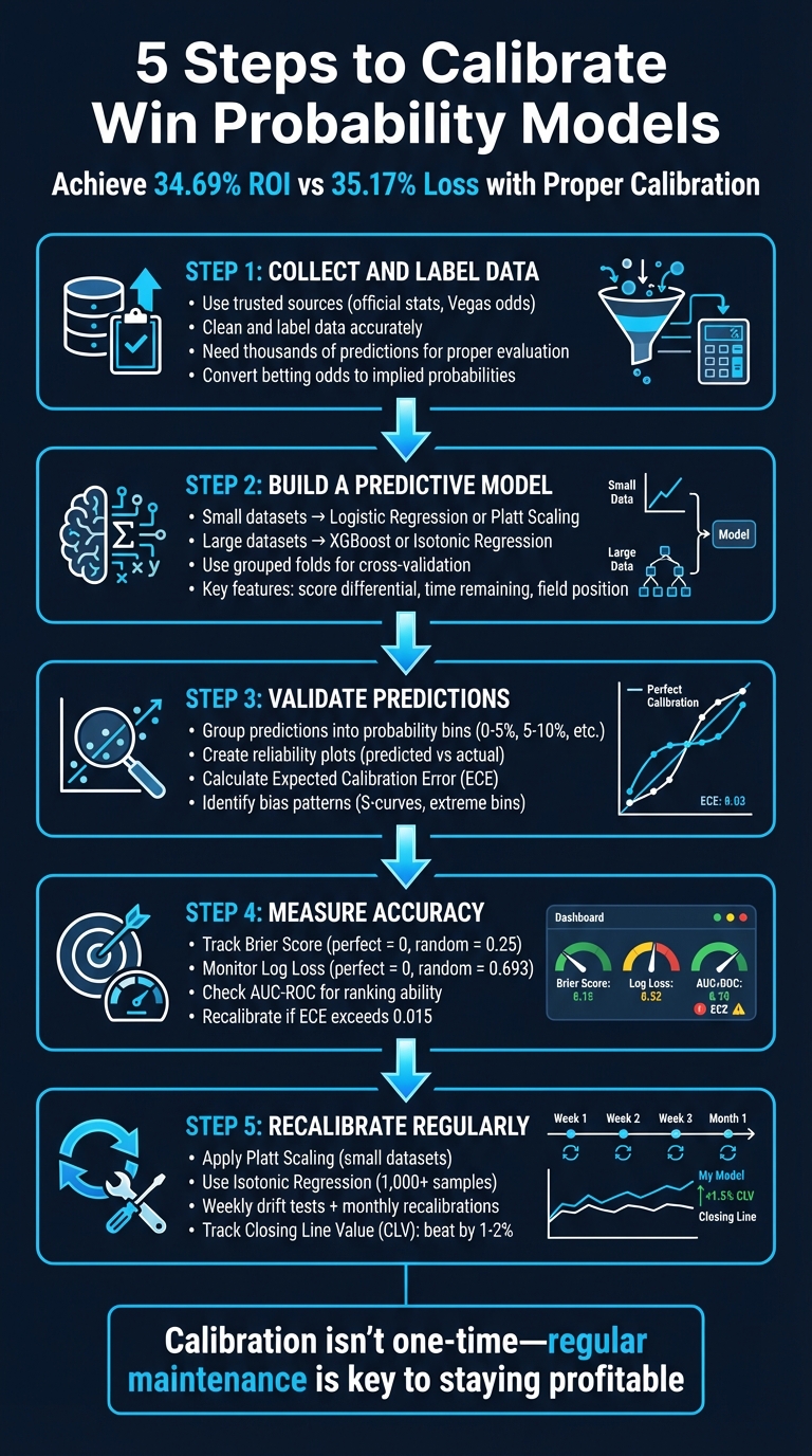
5 Steps to Calibrate Win Probability Models

When your win probability model says "70% chance of winning", does it actually happen 70% of the time? If not, your model may be miscalibrated, leading to poor betting decisions and unnecessary losses. Calibration ensures that predicted probabilities align with real-world outcomes, making your model reliable and profitable. Here's how to get it right:

Collect and Label Data: Use trusted sources like official stats and market odds. Clean and label data accurately to avoid errors.
Build a Predictive Model: Choose methods like logistic regression or XGBoost, depending on your dataset size and complexity.
Validate Predictions: Use probability bins and reliability plots to check if predictions match outcomes.
Measure Accuracy: Track metrics like Brier Score, Log Loss, and Expected Calibration Error (ECE) to ensure precision.
Recalibrate Regularly: Apply techniques like Platt Scaling or Isotonic Regression to fine-tune probabilities.

Calibration isn't a one-time task. Regular maintenance, backtesting, and monitoring metrics like Closing Line Value (CLV) are key to staying ahead. Miscalibrated models can lead to overconfidence and losses, but properly calibrated ones can deliver ROIs of over 30%. Stay sharp, and let the numbers guide your bets.

5-Step Process to Calibrate Win Probability Models for Sports Betting

Probability Calibration Workshop - Lesson 1

Step 1: Collect and Label Historical Sports Data

Your starting point for calibration is the data you feed into your model. Without precise historical records - like play-by-play details, final outcomes, market data (such as Vegas lines), and situational variables (e.g., scoring margin, time left, possession, down, distance, and field position) - the probabilities your algorithms produce will lack reliability. These game-state variables are crucial for building in-game models that update win probabilities as conditions shift.

Choose Trusted Data Sources

Accuracy begins with where you get your data. Rely on dependable sources like official league stats, historical Vegas odds (both opening and closing lines), and platforms like WagerProof for professional-grade data. Historical point spreads and implied probabilities are particularly important because they reflect the market’s collective judgment and provide a solid baseline for your predictions.

Take the Pro-Football-Reference (P-F-R) Model as an example. It uses a normal random variable with a mean based on the Vegas line and a standard deviation of 13.45, calculated from NFL data spanning 1978–2012. This model also factors in "Expected Points" (EP), which accounts for variables like down, distance, and field position. By doing so, it dynamically adjusts win probabilities as game conditions change. Once you've gathered reliable data, the next step is to label it meticulously to ensure your model learns effectively.

Label Data for Model Training

After collecting your data, proper labeling is critical for training your model. Assign clear outcomes - such as wins, losses, and key situational tags - to your dataset. Betting odds should be converted into implied probabilities, and adjustments should be made for the "vig" (the bookmaker’s margin) to ensure consistency across various sportsbooks. Eliminating duplicate entries and fixing labeling errors is equally important to avoid inaccuracies in your model.

"Clean data is especially important - remove duplicate entries, correct inconsistent labeling, and ensure data is structured in a way your model can interpret."
– UnderdogChance

The size of your dataset also plays a huge role. A few hundred bets might not cut it; you’ll need thousands of predictions to properly evaluate your model’s performance. Play-by-play data often comes in clusters of observations tied to the same outcome. If not managed carefully during labeling, this clustering can reduce your effective sample size and inflate bias and variance. To test your model’s accuracy, compare its predictions against market closing odds. If it repeatedly fails to outperform the closing line, your data or calibration process may need a second look.

Step 2: Build a Predictive Model

Once your data is clean and labeled, it’s time to build your model. The approach you choose should depend on the size and complexity of your dataset. For smaller datasets, methods like logistic regression or Platt Scaling are more reliable because they’re less prone to overfitting. However, if you’re working with a larger dataset that includes complex interactions, tools like XGBoost (Extreme Gradient Boosting) or Isotonic Regression are better suited to handle the challenge. XGBoost, in particular, excels at managing non-linear relationships and allows for monotone constraints - a feature that ensures, for instance, that increasing a lead will never decrease the win probability. The key is to align your model selection with the characteristics of your data.

Select the Right Modeling Approach

Your goal is to find a model that strikes a balance between accuracy and calibration. Why does calibration matter? Because well-calibrated models can significantly improve ROI. For instance, a well-calibrated model can deliver an ROI increase of +34.69%, while an overly accuracy-focused model might result in a 35.17% loss. XGBoost stands out here, as it allows you to enforce logical constraints, like ensuring that increasing a lead doesn’t reduce win probability.

When validating your model, use grouped folds for cross-validation. This ensures that all plays from a single game stay within the same fold, preventing "leakage" - where the model might learn from future plays it shouldn’t have access to. Keep complexity in check to avoid overfitting. For example, in a college football model, reducing the max_depth parameter in XGBoost from 20 to 5 reduced calibration error by 75%. This shows how simplifying your model can often lead to better results.

Engineer Features for Accuracy

Once you’ve selected your modeling framework, focus on creating precise and meaningful features. Key variables include score differential, time remaining, field position (yards to the opponent’s goal), down, distance to go, and timeouts remaining for both teams. Possession is another critical factor, as having the ball can significantly shift win probability, especially in high-scoring sports.

You can also incorporate pregame point spreads, but make sure to adjust their influence as the game progresses. A time-decay function like new_spread = spread * (clock_in_seconds/3600)^3 can help reduce their weight over time. When play clock data isn’t reliable, consider using the percentage of the game completed based on play counts. Additionally, engineering synthetic end-of-game rows to force win probabilities to converge to 0% or 100% at the final whistle ensures your model aligns with the actual flow of a game. These feature adjustments help your model mirror the dynamics of real games, setting the stage for validating predictions through probability bins.

Step 3: Validate Model Predictions Using Probability Bins

Once you've built your model and engineered features, it's time to validate how well your predictions align with actual outcomes. Start by grouping your predicted probabilities into probability bins - ranges like 0–5%, 5–10%, and so on. Then, compare these grouped predictions to the actual results. For example, if your model predicts a 70% chance of winning, you’d expect that team to win about 70% of the time when grouped alongside similar predictions. This step helps highlight whether your model tends to be overly confident or too cautious.

You can use two common binning methods: fixed-width binning or equal-frequency (quantile) binning. Fixed-width binning divides the probability range into equal intervals, making interpretation straightforward. On the other hand, equal-frequency binning organizes predictions into bins with an equal number of observations, which is especially helpful if your model rarely predicts within certain ranges. A typical approach is to use 10 fixed bins for calibration metrics, though a general guideline suggests the optimal number of bins is around the cube root of your total predictions.

Create Reliability Plots

A reliability plot (or calibration plot) is a handy visual tool for assessing your model’s calibration. To create one, plot the average predicted probability (x-axis) against the actual win rate (y-axis) for each bin. Ideally, all points should fall on the 45-degree diagonal line, where predicted probabilities match observed outcomes.

If points fall below the diagonal, your model is overestimating probabilities, while points above it indicate underestimation. Using quantile binning to create deciles ensures that each bin has enough data points for meaningful averages. These plots are a great way to identify trends before diving deeper into potential biases.

Identify Bias in Model Predictions

After creating your bins and plotting them, look for patterns that might reveal systematic biases. Pay close attention to extreme probability bins (e.g., below 15% or above 85%). If predictions in these high-confidence bins tend to move toward the center of the plot, it could indicate over-regularization or missing important features. Another common pattern is an S-shaped curve, where the model is overly confident at the extremes but less confident in the middle ranges. For instance, if predictions between 35% and 65% consistently fall below the diagonal, it suggests overconfidence in uncertain scenarios.

To measure these discrepancies, calculate the Expected Calibration Error (ECE), which averages the absolute differences between predicted and actual frequencies, weighted by the number of observations in each bin. Keep in mind that calibration analysis works best with large datasets - thousands of predictions are often needed to draw reliable conclusions. These calibration checks set the stage for assessing model accuracy with key metrics in the next step.

Step 4: Measure Model Accuracy With Key Metrics

Once you've validated your model's predictions using probability bins and reliability plots, the next step is to quantify its performance with metrics that evaluate both discrimination and calibration. Accurate measurement is essential to ensure your model aligns with the realities of sports betting. Let’s dive into two key calibration metrics and see how they compare to discrimination measures.

Brier Score and Log Loss

The Brier Score calculates the mean squared difference between predicted probabilities and actual outcomes. In simpler terms, it measures how close your predictions are to reality. It’s computed as the average of ((\text{predicted probability} - \text{actual outcome})^2) across all predictions. A perfect score is 0, while a random model typically scores around 0.25. For sports betting, staying well below 0.25 is critical - anything close suggests your model isn’t adding much value.

Log Loss, or cross-entropy, works a bit differently. It uses logarithmic penalties to harshly punish overconfident but incorrect predictions. While a perfect score is 0, a random model often hovers around 0.693. For instance, if your model predicts a 99% chance of a team winning, but they lose, the Log Loss spikes to 4.6052. This metric forces models to balance confidence with accuracy.

A 2024 study from the University of Bath, published in Machine Learning with Applications, analyzed NBA betting models over an entire season. It found that models selected based on calibration metrics outperformed those chosen purely for raw accuracy. Calibration-based models yielded an average ROI of +34.69%, compared to -35.17% for accuracy-based selections. The best-calibrated models even reached an ROI of +36.93%. On the flip side, if your Expected Calibration Error (ECE) exceeds 0.015 during weekly tracking, it’s a clear indicator that recalibration is needed.

Area Under the Curve (AUC)

While Brier Score and Log Loss focus on the accuracy of your probability estimates, AUC-ROC (Area Under the Curve - Receiver Operating Characteristic) measures how well your model ranks outcomes. Specifically, it evaluates whether your model can distinguish between winners and losers. AUC scores range from 0 to 1, with higher scores indicating better ranking ability.

However, a high AUC doesn’t necessarily mean your model is well-calibrated. For example, your model might rank one team higher than another with probabilities of 85% and 80%, but if the true probabilities are closer to 65% and 60%, those overconfident predictions could lead to poor betting decisions.

Step 5: Fine-Tune and Recalibrate the Model

Once you've completed your calibration checks, the next step is to fine-tune the model outputs for better alignment with practical scenarios. Even models with a high AUC can sometimes misrepresent confidence levels, so recalibrating probabilities is essential. Two widely used techniques for this are Platt Scaling and Isotonic Regression.

Platt Scaling applies a logistic regression model to the raw outputs, making it a good choice for smaller datasets or when dealing with sigmoid-shaped miscalibrations. To use this method, you first need to convert probabilities into log-odds using the formula:
$z = \log(p / (1-p))$.
This step ensures the data aligns with logistic regression assumptions.
Isotonic Regression is better suited for larger datasets (1,000+ samples) and more complex miscalibrations. It provides a flexible way to correct monotonic distortions without assuming a specific functional form.

When using either method, it’s crucial to train the calibration model on a separate validation set to avoid introducing bias.

Adjust for Multicollinearity

Redundant features can throw off your model's calibration, especially when they push probabilities toward extreme values like 0 or 1. For instance, features such as "points per game" and "offensive efficiency rating" often carry overlapping information. To address this, calculate correlation coefficients between features and either remove or combine highly correlated ones into composite metrics. This ensures cleaner, more balanced inputs, leading to more reliable probability estimates.

Backtest Across Seasons

To verify your model's consistency over time, use rolling window validation. For example, train the model on data from 2018–2020 and validate it using data from 2021–2023. This method helps you identify whether the model holds up across different time periods.

During backtesting, keep an eye on metrics like the Brier Score and Expected Calibration Error (ECE). If your ECE exceeds 0.015 during weekly evaluations, it’s time to re-fit your calibration mappings. Additionally, monitor your Closing Line Value (CLV) - a well-calibrated model should consistently beat the closing line by 1%–2%. These checks ensure your model remains accurate and effective over time.

Monitor and Maintain Calibration Over Time

Keeping your model calibrated isn’t a one-and-done task. Betting markets, team dynamics, and public sentiment are always shifting, which means a model that worked perfectly last season could fail this year. Just like a car needs regular tune-ups, your model requires consistent attention to stay effective.

Create a structured schedule for maintenance. Include weekly drift tests (using tools like KS or Kuiper tests) and monthly recalibrations if the Expected Calibration Error (ECE) exceeds 0.015. Additionally, plan for a full model retrain each season to account for changes like roster updates, coaching strategies, or rule adjustments. These proactive measures ensure your model stays ready for the evolving landscape.

Keep an eye on Closing Line Value (CLV) to detect long-term drift. If your model consistently misses the closing line by 1%–2%, it’s a clear sign that your probabilities are slipping out of sync. Another telltale sign is a growing gap between raw and calibrated probabilities, so make sure to log both for ongoing analysis.

For live betting models, the stakes are even higher. Since real-time variables can shift quickly, you’ll need to increase your monitoring frequency accordingly. Automate alerts to flag any breaches in key metrics, so you can act immediately when something goes off track.

Platforms like WagerProof can make this process smoother. They offer real-time data feeds and automated tools for spotting outliers, helping you catch when your predictions stray from market consensus. These tools also provide value bet signals and highlight mismatches in prediction markets, giving you an extra layer of validation for your calibration efforts.

Conclusion

Fine-tuning win probability models plays a crucial role in managing risk and maintaining profits over time. To achieve this, focus on these five steps: data collection, model building, prediction validation, accuracy measurement, and continuous recalibration.

The numbers back it up. A study by Conor Walsh and Alok Joshi, published in June 2024, highlights the stark difference calibration can make. Calibration-based models showed a 34.69% ROI, compared to a 35.17% loss for models that prioritized accuracy alone. That nearly 70-point swing proves how vital it is to have confidence levels that reflect reality.

"Accuracy tallies wins, calibration reveals the true odds, enabling smarter betting strategies, better risk management, and sustainable profits." - Adam Wickwire, OpticOdds

This underscores the importance of treating calibration as an ongoing process. Markets evolve - team rosters change, public sentiment shifts, and past patterns don't always predict future outcomes. Without regular recalibration, even the best models can fall behind. Tools like WagerProof simplify this process by offering real-time data feeds and automated alerts whenever your predictions stray from market trends. Staying calibrated is the key to staying ahead.

FAQs

How many predictions are needed to trust calibration results?

When it comes to achieving reliable calibration, the number of predictions needed can vary depending on the situation. However, as a general rule, larger sample sizes lead to better accuracy. Techniques such as reliability diagrams or cumulative difference plots work best when applied to hundreds or even thousands of predictions. This larger dataset makes it easier to spot miscalibration and ensures the estimates are more stable.

When should I use Platt Scaling vs Isotonic Regression?

When deciding between calibration methods, Platt Scaling is a great choice if you're looking for a parametric approach. It assumes a sigmoid-shaped relationship between predicted scores and true probabilities. This method is especially effective when working with models like SVMs or boosted trees, and it performs well even with smaller datasets.

On the other hand, Isotonic Regression offers a non-parametric alternative. It’s designed to handle more complex and irregular relationships that don’t fit a sigmoid curve. This flexibility makes it a better fit for larger datasets or scenarios where calibration curves are less predictable.

How do I know my model is drifting during the season?

Regularly checking your model’s calibration is crucial to ensure it stays reliable. Calibration essentially measures how closely the predicted probabilities align with real-world outcomes. To do this, you can monitor metrics like the Brier Score, Expected Calibration Error (ECE), or use reliability curves.

If you notice these metrics getting worse or deviating significantly, it could be a sign of drift. Another way to spot issues is by comparing predicted probabilities against actual outcomes over time. Any noticeable discrepancies might indicate your model is becoming miscalibrated.