
How to Test Model Robustness in Betting
Testing your betting model's reliability is more than just running basic backtests. A strong model performs consistently across various conditions, like new seasons, unexpected events, or market shifts. Here's what you need to know:
- Avoid Overfitting: Models often fail because they latch onto random patterns in historical data instead of genuine trends. This leads to poor performance when conditions change.
- Go Beyond Basic Backtesting: Standard backtests miss real-world factors like market friction (commissions, slippage) and look-ahead bias. Advanced methods are needed to evaluate performance under uncertainty.
- Methods to Test Reliability:
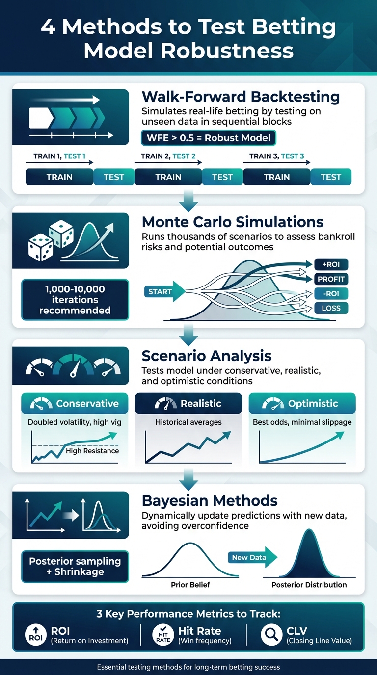
- Walk-Forward Backtesting: Simulates real-life betting by testing on unseen data in sequential blocks.
- Monte Carlo Simulations: Runs thousands of scenarios to assess bankroll risks and potential outcomes.
- Scenario Analysis: Tests the model under conservative, realistic, and optimistic conditions to gauge sensitivity to changes.
- Bayesian Methods: Dynamically update predictions with new data, avoiding overconfidence in limited samples.
Key metrics like ROI, hit rate, and Closing Line Value (CLV) help measure performance. Tools like WagerProof simplify testing by combining live data, simulations, and automated outlier detection, ensuring your model can handle uncertainty and deliver consistent results.
4 Methods to Test Betting Model Robustness
How To Implement Robustness Testing In Trading Backtests For Better Results (5/7) | Quantreo

Why You Need to Test Model Robustness
Many betting models fail not because of poor design, but because they mistake random noise for meaningful patterns. When you build a model using historical data, there’s always a risk of picking up on temporary anomalies - like a short injury streak or unusual weather - rather than genuine, repeatable trends.
The Risks of Overfitting in Betting Models
Overfitting is one of the biggest traps in model building. It gives you the illusion of having an edge. Your backtests might look incredible, but once you start betting for real, the results often fall apart. Why? Because the model has essentially memorized quirks in the historical data rather than learning the actual dynamics of the game.
"A good model can lose due to variance. An overfitted model will lose because it was flawed from the start." - TheOver.AI
This distinction is critical. Variance is the short-term randomness that can cause you to lose a few bets even if your model has a solid edge. Overfitting, on the other hand, leads to long-term failure because the model wasn’t built to handle real-world changes. When rules change, teams evolve, or markets become more efficient, an overfitted model collapses. Warning signs include performance that drops sharply when tested on new seasons or leagues - clear evidence the model latched onto specific, non-transferable patterns in the data.
While overfitting erodes your model’s reliability, relying solely on basic backtesting can also leave you blind to critical issues.
Why Basic Backtesting Isn't Enough
Even if your backtests look promising, they might not tell the whole story. Standard backtesting often overlooks real-world constraints like market friction and look-ahead bias. Market friction includes things like commissions, vig, liquidity limits, and slippage - factors that can eat into your profits but are rarely accounted for in basic tests. Look-ahead bias, on the other hand, occurs when your model accidentally uses future data to predict past outcomes, creating results that are too good to be true.
"Backtesting is not a guarantee of profit but when executed correctly it becomes a central part of disciplined data driven betting." - Great Bets
Short-term patterns in historical data can create the illusion of statistical significance, but these patterns often don’t hold up over time. This is where robustness testing comes in. It pushes your model to prove itself under different scenarios, with unseen data, and while accounting for real-world challenges - not just by analyzing wins and losses in cherry-picked historical datasets.
Setting Up a Backtesting Framework
Building a backtesting framework involves three key components. First, you need a backtesting engine - software that uses historical data and your betting logic to simulate how your model would have performed in the past. This includes defining a starting bankroll and creating specific betting algorithms to test. Second, you'll need PnL (Profit and Loss) calculation logic that reflects real-world costs. For instance, if you're testing a model for exchange betting, you must account for commission fees, like Betfair's 5% charge on winnings, and slippage - the gap between the expected price and the actual price you get. Third, apply out-of-sample validation to test your model on data it hasn’t encountered before. Methods like train-test splits or rolling window validation ensure your model is evaluated under conditions closer to reality. Once these components are in place, the quality of your data becomes a critical factor.
High-quality data underpins any effective backtesting framework. You’ll need real-time sports data platforms for official league feeds for schedules, rosters, and box scores, which should be updated daily for basic stats and in real time for live scores. Historical stats should also refresh daily, typically within 3–4 days after games to maintain accuracy. Real-time odds feeds are essential for tracking line movements and sharp money, with sub-minute updates via WebSocket feeds to capture rapid market changes.
It’s also important to simulate execution conditions rather than assuming perfect trades. For example, a robust backtesting engine should replicate Betfair Exchange conditions by factoring in the 5% commission and using the best available kick-off odds. This avoids the common mistake of assuming you can always execute bets at the last known price, which ignores the potential market impact of large stakes.
Additionally, consider liquidity and stake constraints. Use maximum limits and rolling-window simulations to mimic how your bets might affect the market in real time. Rolling windows force your model to continuously adapt, just as it would need to in live betting scenarios.
Finally, implement a stop-loss mechanism within your backtesting process. If your model's calibration or closing line value (CLV) performance declines over a rolling window of 500–1,000 games, pause the process to investigate potential data issues or shifts in market behavior. This approach, combined with continuous monitoring, helps ensure your model remains robust even as market conditions evolve.
Walk-Forward Backtesting
Walk-forward backtesting tackles a common flaw in traditional backtesting: data leakage. In standard setups, models are often trained on a continuous stretch of historical data - like training on data from 2020 to 2024 and testing on 2025. But this doesn’t reflect real-life betting, where future data isn't available. Walk-forward analysis solves this by splitting the dataset into sequential blocks. It trains on an in-sample (IS) period, tests on an out-of-sample (OOS) period, and then shifts these windows forward iteratively, simulating real-world conditions where bettors adjust to new data as it becomes available.
Here’s how it works: Train your model on an initial set of games, test it on the next segment, and then slide the window forward. Repeat this process at least 10 times to ensure your strategy is exposed to various market conditions.
One key metric in this method is the Walk-Forward Efficiency (WFE), which compares the out-of-sample Sharpe Ratio to the in-sample Sharpe Ratio. A WFE above 0.5 signals that the strategy retains at least half of its in-sample performance when tested on unseen data. If the WFE approaches 1.0, it indicates the model generalizes exceptionally well to live betting scenarios.
"WFE above 0.5 indicates robustness; the strategy retains at least half its in-sample performance when faced with unseen data." - Nicolae Filip Stanciu
To avoid overfitting, reserve the most recent data as a blind test set, which should only be used after finalizing your model's logic and parameters. This step acts as a safeguard against over-optimization, where a model might excel in historical tests but fail in live betting. By keeping this blind test untouched until the end, you ensure a more realistic evaluation of your strategy. This iterative approach aligns with the broader backtesting framework, offering a more reliable way to assess performance.
Key Metrics for Measuring Model Performance
Once you've wrapped up walk-forward backtesting, it's time to dig into the numbers that reveal how your model truly performs under market pressures. The most important metrics to evaluate include Return on Investment (ROI), hit rate, and Closing Line Value (CLV). Each one highlights a different dimension of your betting model's effectiveness, helping you identify whether your model's success is genuine or merely a result of overfitting to past data.
ROI measures your net profit or loss as a percentage of your total wagers. While it’s a straightforward way to gauge profitability, ROI can be heavily influenced by short-term variance. A lucky streak of wins might temporarily inflate your ROI, making a flawed model appear successful. Hit rate, on the other hand, tracks how often your bets win. But this metric alone can be deceptive - it doesn’t account for the odds. For instance, consistently winning bets on low-odds favorites might yield a high hit rate but generate less profit than a lower hit rate on high-odds underdogs.
Closing Line Value (CLV) is another critical metric. It measures the difference between the odds you bet at and the final market odds. The closing line represents the collective knowledge of the market, factoring in late-breaking news like injuries, weather updates, and sharp betting activity. This makes it a strong indicator of the "true" probability of an event. If you regularly place bets at better odds than the closing line, it suggests you have a legitimate edge. For context, in highly competitive markets like NFL spreads, a consistent CLV of +2% to +3% is considered outstanding.
"The closing line is the receipt that proves you got a discount. Stop celebrating wins that had negative CLV - those are bad habits rewarded by luck." - EdgeSlip
To get the full picture, track these metrics together. CLV reflects your expected outcomes, while ROI shows your actual results. If your CLV remains positive but your ROI is negative, it’s likely a matter of variance, and over time, as your sample size grows, your ROI should align more closely with your CLV. Additionally, Expected Value (EV) provides another layer of insight by estimating potential returns. EV is calculated as: (win probability × win amount) minus (loss probability × loss amount). A positive EV indicates that your bets are mathematically profitable opportunities.
Stress Testing with Monte Carlo Simulations
How to Simulate Betting Scenarios
Monte Carlo simulations are a powerful way to test the durability of your betting model, providing insights into how your bankroll might perform under thousands of possible outcomes. To get started, you'll need to define a few key inputs: your estimated win probability (independent of sportsbook odds), the odds offered by the sportsbook, your stake size (either a fixed dollar amount or a percentage of your bankroll), your total bankroll, and the number of bets you'll place over a season.
You can use Excel's RAND() function to simulate outcomes. If the random number generated is below your predicted win probability (e.g., 0.58 for a 58% chance), it counts as a win. By running this process for at least 1,000 to 10,000 iterations, you can create a reliable distribution of potential outcomes. For example, a study running 100,000 iterations revealed that actual profit (0.76%) was surpassed in 78% of scenarios, illustrating how variance can lead to underperformance.
This method complements earlier evaluation techniques by quantifying potential losses and emphasizing the importance of a well-tested model. Don't forget to account for market friction, like the vig. For instance, when betting on standard -110 lines, a win adds $1 to your bankroll, but a loss subtracts $1.10.
"The Monte Carlo method relies on repeated random sampling to obtain numerical outputs when other mathematical approaches would prove to be too complicated."
Joseph Buchdahl, Betting Analyst at Pinnacle
Once you've generated your simulation results, the next step is to analyze the distribution and understand the range of possible outcomes.
Analyzing Bankroll Distributions
Instead of focusing solely on averages, pay attention to percentile outcomes, which provide a clearer picture of best- and worst-case scenarios. For example, the 5th and 95th percentiles show realistic extremes for your bankroll. In professional simulations using historical win rates, median profits were +2.1 units, but the 5th percentile dropped to -21 units. In another case, the 90th percentile showed a 35% bankroll growth, while the 10th percentile reflected an 18% loss - highlighting how variance can still affect results, even with a positive edge.
Another key metric is the probability of ruin, which measures how often your bankroll would hit zero in the simulations. For instance, in a case study of 500 bets with a 4% edge, flat staking kept the ruin probability below 1%. However, switching to a 2% variable staking strategy increased the average return but pushed the ruin probability above 8%.
You should also track the Expected Maximum Drawdown (EMDD), which represents the average largest drop in your bankroll from a peak over a series of bets. If your EMDD exceeds 30 units or your ruin probability climbs above 25%, it’s time to lower your bet sizes - say, from 3% to 2% of your bankroll - to maintain long-term sustainability. These insights can help you fine-tune your staking strategy and betting model as you move forward.
Scenario Analysis for Real-World Testing
Building on the insights gained from simulations, scenario analysis takes things a step further by evaluating how a model behaves when subjected to deliberately altered conditions.
Testing Conservative, Realistic, and Optimistic Scenarios
Scenario analysis isn't just about replaying historical data - it’s about pushing your betting model into different hypothetical situations to see how it holds up. To do this, you can define three primary scenarios: conservative, realistic, and optimistic. These scenarios help you understand how sensitive your model is to changes in key variables.
In a conservative scenario, you might double historical volatility, raise the vig to 1% or more, and force correlations close to 0.95. This simulates challenging conditions, like a spike in injuries or weather disruptions that skew results.
A realistic scenario uses historical averages as the baseline. It assumes standard injury rates, typical market conditions, and usual commission levels - essentially, the day-to-day environment your model is likely to encounter.
On the other hand, an optimistic scenario assumes everything goes your way: minimal slippage, access to the best odds, and a roster of perfectly healthy players.
For even more rigorous testing, you can simulate extreme events, like a sudden 30%–35% drop in odds (a flash crash), to see if your bankroll management and stop-loss mechanisms can handle abrupt market shifts. Gradual performance decline during these tests is expected, but a sharp collapse might point to overfitting.
By testing these scenarios, you can compare how critical performance metrics respond to different conditions.
Comparing ROI and Risk Metrics Across Scenarios
Once you’ve run your scenarios, it’s time to analyze the results. Use metrics like ROI, median ROI, maximum drawdown, and the Sharpe ratio (which measures returns relative to volatility). A durable model should show slightly positive ROI under realistic and optimistic conditions, while the conservative scenario might hover near breakeven or dip slightly negative - but without catastrophic losses.
Here’s an example of how to organize your findings:
| Scenario Type | Modified Inputs | Expected Outcome |
|---|---|---|
| Conservative | 1%–2% commission, doubled volatility, high correlations, increased injury rates | ROI near breakeven or slightly negative, high drawdown, and lower Sharpe ratio |
| Realistic | Historical average odds, standard injury rates, typical vig | Modest positive ROI with moderate drawdowns and balanced risk metrics |
| Optimistic | Best available odds, minimal slippage, peak player health | Higher positive ROI, lower drawdowns, and improved risk-adjusted returns |
If the conservative scenario shows a particularly high drawdown or a sharp drop in the Sharpe ratio, it might be worth introducing a regime filter to sideline your model during periods of extreme volatility. This kind of structured analysis not only helps you assess the level of risk your model is taking but also confirms whether it can maintain its edge as conditions change. It ties back to the broader goal of ensuring your model is built for long-term success.
Using Bayesian Methods to Manage Uncertainty
Bayesian methods take scenario analysis to the next level by dynamically updating probability estimates as new information comes in. Unlike traditional models that offer a single, static probability (like a 55% chance of winning) without accounting for confidence levels, Bayesian methods treat probabilities as evolving beliefs. These beliefs adjust with new evidence - whether it’s player injuries, weather changes, or shifts in team performance. Instead of a fixed number, you get a posterior distribution that reflects the full range of uncertainty in your prediction. This approach is especially useful when data is limited. For example, if a team has only played three games under a new coach, the model leans on its prior assumptions, avoiding overconfidence in conclusions drawn from sparse data. Essentially, Bayesian methods transform raw data into dynamic probabilities, expected values, and scalable position sizes.
Posterior Sampling for Expected Value (EV) Distributions
Posterior sampling allows you to draw thousands of probability samples from the posterior distribution and plug them into your betting formula. For each sample (p), you calculate the expected value (EV) using the formula:
EV = p(d − 1) − (1 − p) (where d represents decimal odds).
This process generates a full distribution of potential EVs, showing you the likelihood of having an edge - defined as the proportion of the EV distribution above zero. A bet is placed only if the probability of EV > 0 crosses a certain threshold, such as 60% or 70%. This method incorporates Bayesian risk control into decision-making.
It also supports a more flexible staking strategy. Instead of sticking to a fixed Kelly fraction, you can integrate over the posterior distribution to determine a range of possible Kelly stakes. By using a conservative quantile, like the 25th percentile, you can scale down bets when uncertainty is high. This approach helps manage risk while accounting for the inherent unpredictability in the data.
Using Shrinkage to Avoid Overreaction
Short-term results can be misleading. Winning three games in a row doesn’t necessarily mean a team is performing at an elite level. Shrinkage, or partial pooling, addresses this by pulling extreme or noisy estimates closer to a stable, league-wide average. This prevents the model from overreacting to temporary streaks or slumps.
Empirical Bayes is a particularly effective tool for this. By using historical league-wide data to estimate a prior, it stabilizes predictions - especially early in a season when sample sizes are small. For instance, if a team starts the season 5–0, shrinkage keeps the model from assigning an overly high win probability. Instead, it tempers the estimate by borrowing information from the league average.
This technique is a key safeguard against overfitting. Models that seem flawless in backtesting often fail in live markets because they overreact to random variance in the training data. Shrinkage helps maintain balance, ensuring predictions remain grounded even in the face of short-term fluctuations.
Using WagerProof for Robustness Testing

WagerProof simplifies the process of testing your betting model's robustness by combining real-time data with automated analysis. Instead of creating complex simulation frameworks, you can use its platform to validate your model through live data, including prediction markets, historical stats, public betting trends, and statistical models - all in one place. This allows you to stress test your model dynamically, moving beyond static backtests to a more practical, real-time approach.
Using WagerBot Chat for Live Simulations
WagerBot Chat stands out as an AI tool for sports betting that connects directly to real-time professional data while ensuring accuracy. It enables live simulations by analyzing prediction markets, odds discrepancies, and historical stats in real time, helping to test your model under changing conditions. For instance, it can simulate over 1,000 equity curves for upcoming NFL games by sampling live odds, which helps assess how your bankroll might react to volatility.
This feature is particularly useful for spotting how your model performs during unexpected market shifts - like a betting line moving from -3 to -6 without valid statistical reasoning - before you commit real money.
Additionally, WagerBot Chat automates walk-forward backtesting. By pulling real-time historical data for rolling windows, it lets you re-optimize your model using the most recent in-sample data (e.g., the last 70% of games) and then test it on unseen live odds. Running this process across 1,000+ iterations minimizes the risk of overfitting and aligns with the principles of randomized out-of-sample testing. To further refine accuracy, WagerProof incorporates automated tools for detecting outliers.
Applying Automated Outlier Detection Tools
WagerProof’s outlier detection tools are designed to spot mismatches and contrarian signals by comparing current prediction market spreads to historical data. For example, if an NBA game’s implied win probability from the odds is 55%, but your model calculates it as 62%, the platform may flag this as a potential value bet. You can then run simulated bets on these discrepancies to test your model's performance under such scenarios.
These flagged outliers can also feed into Monte Carlo simulations, providing deeper insights into potential risks. This approach allows for stress testing against worst-case scenarios, revealing drawdowns that may exceed standard backtest limits by 20–30%.
Integrating Pro-Level Data and Analysis
WagerProof takes testing a step further by incorporating expert-vetted picks alongside its pro-level data. This enhances the management of Bayesian uncertainty. By feeding live market data into posterior sampling, WagerProof applies adjustments based on expert insights. For instance, an NFL spread prediction might initially suggest a 65% win probability, but real-time data and expert input could adjust this to 58%, offering a more realistic evaluation of your model’s robustness under degraded conditions.
Unlike manual backtesting, which can fall prey to data snooping, WagerProof automates precision checks. For example, it ensures a 61% true positive rate on model predictions and evaluates ROI across varying scenarios - conservative, realistic, and optimistic. By leveraging live data to prevent overfitting, the platform uncovers hidden opportunities and can improve long-term returns by 2–5%. This detailed, real-time approach ensures your model can handle uncertainty while maintaining reliability over time.
Conclusion: Testing for Long-Term Success
Creating a reliable betting model isn’t just about crunching numbers - it’s about ongoing, thorough validation. Walk-forward backtesting helps you see how your model performs over time, simulating real-world use. Monte Carlo simulations give you a glimpse into how your bankroll might behave under extreme scenarios. Scenario analysis helps you weigh conservative, realistic, and optimistic outcomes before committing capital. And Bayesian methods, like posterior sampling, help handle uncertainties in expected value, preventing overreactions to short-term changes. These strategies form a strong foundation for platforms like WagerProof to keep your model sharp and effective.
With these methods in place, WagerProof simplifies the testing process by integrating real-time data, automated detection of outliers, and live simulations through its WagerBot Chat. Instead of building complex systems from scratch, you can validate your model dynamically using prediction markets, historical stats, and expert-approved picks - all in one place. The platform identifies value bets, runs thousands of simulated scenarios, and monitors key metrics to ensure your model consistently beats the market.
FAQs
How do I know if my model is overfitting?
To identify overfitting, look for a model that performs exceptionally well on historical data but falters when applied to new data. This issue often appears as high accuracy during backtesting but poor performance on future predictions. One way to address this is by using cross-validation, which allows you to compare results across training and validation datasets. If the model's performance is significantly better on the training data, overfitting is likely. Additionally, keeping an eye on metrics like Brier Score or Log Loss can help detect predictions that are overly confident and less reliable.
What costs should I include in a realistic backtest?
When testing sports betting models, it's crucial to factor in costs that align with actual betting conditions. These costs can significantly impact your results and help create a more realistic picture. The main ones to consider include:
- Vig or commission: This is the bookmaker's margin, which directly cuts into your potential profits.
- Transaction costs: These are fees associated with placing bets or moving funds between accounts.
- Market impact or slippage: Odds or market conditions can shift before your bet is executed, which can affect the outcome.
Taking these into account ensures your backtest mirrors real betting scenarios, preventing overly optimistic profitability estimates.
How much CLV is enough to trust my edge?
A Closing Line Value (CLV) that consistently outperforms the market by 1-2% is a solid sign of a dependable betting advantage. If you can maintain positive CLV over a large number of bets, it indicates that your wagers are beating the closing odds - a key factor linked to long-term success. Strive for steady positive CLV, as it reflects a reliable edge and reinforces confidence in your overall betting approach.
Related Blog Posts
Ready to bet smarter?
WagerProof uses real data and advanced analytics to help you make informed betting decisions. Get access to professional-grade predictions for NFL, College Football, and more.
Get Started Free