Top Hyperparameters for Sports Betting Models
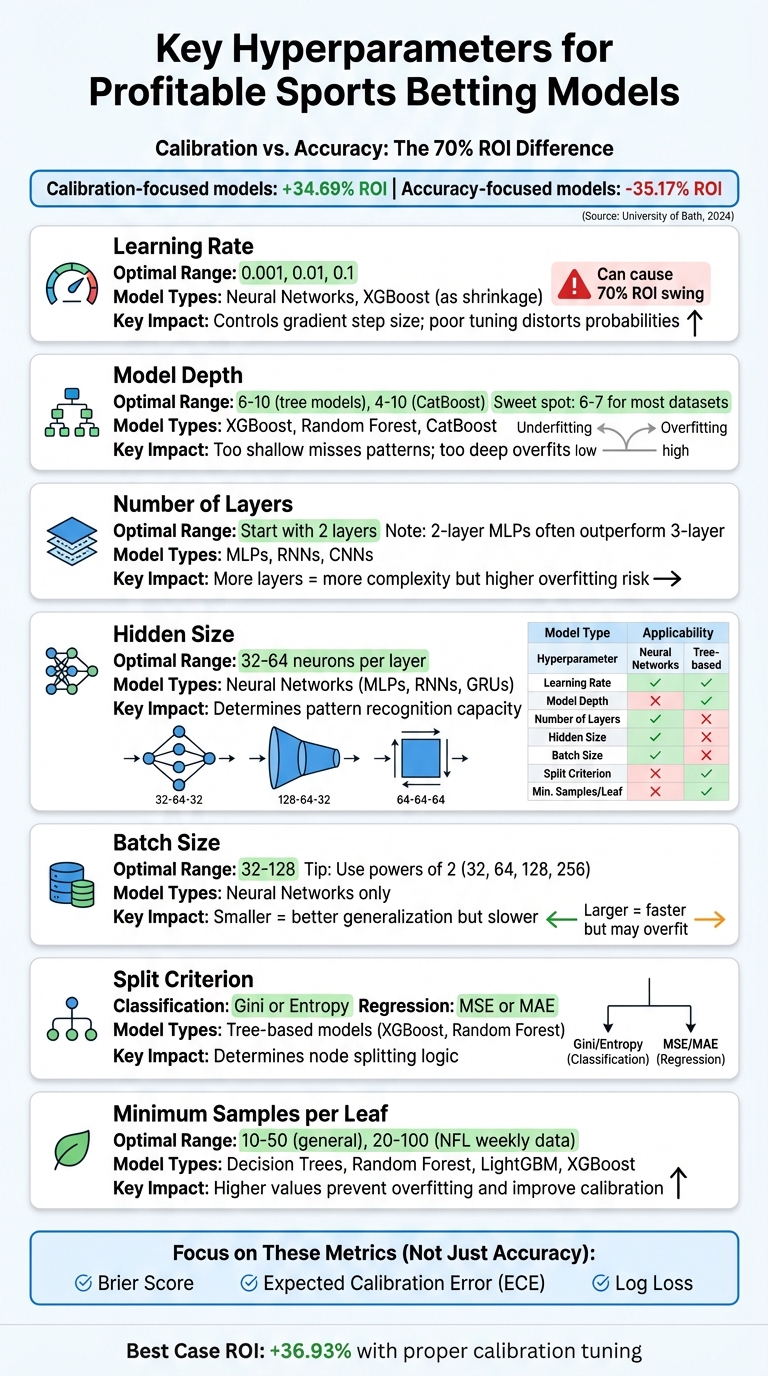
Hyperparameter tuning is the key to making sports betting models profitable. It’s not just about accuracy; calibration - how well predicted probabilities match actual outcomes - has a bigger impact on your return on investment (ROI). A University of Bath study found that calibration-focused models delivered a 34.69% ROI, while accuracy-focused models led to a 35.17% loss. Here’s what you need to know:
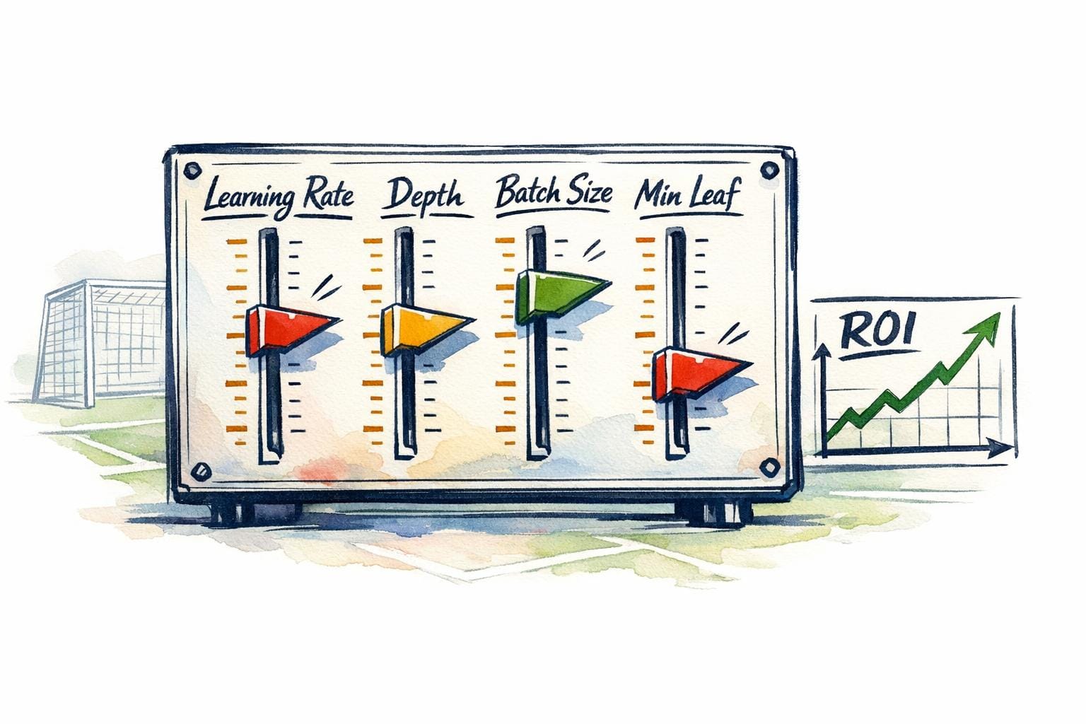
- Learning Rate: Controls how much models adjust during training. Start with 0.001, 0.01, or 0.1. Poor tuning can distort probabilities, leading to overconfidence and losses.
- Model Depth: Too shallow misses patterns, too deep risks overfitting. For tree models, aim for a max depth of 6–10.
- Number of Layers: For neural networks, start with 2 layers. More layers can improve predictions but risk overfitting.
- Hidden Size: Use 32–64 neurons per layer for balanced performance in neural networks.
- Batch Size: Smaller batches (32–128) help generalization but slow training; larger batches train faster but may overfit.
- Split Criterion: For tree-based models, choose Gini or Entropy for classification, and MSE or MAE for regression tasks.
- Minimum Samples per Leaf: Set higher values (e.g., 10–50) to avoid overfitting and improve calibration.
Key Takeaway: Focus on calibration, not just accuracy. Use metrics like Brier Score and Expected Calibration Error (ECE) to fine-tune hyperparameters for better betting strategies.
Sports Betting Model Hyperparameters: Optimization Ranges and Impact Guide
Learn Optuna with Baseball Data | Classifying MLB Pitch Types with Machine Learning

1. Learning Rate
Choosing the right learning rate is a critical step in training any model effectively. The learning rate determines how much the model adjusts its weights during each training iteration. Essentially, it controls the size of the gradient step. If the learning rate is too high, the model may oscillate wildly without converging. On the other hand, if it's too low, training can drag on endlessly or settle into a less-than-ideal solution.
Impact on Model Accuracy
The learning rate doesn’t just dictate how quickly a model trains - it also plays a big role in how well the model aligns its predictions with real outcomes. For example, a model might predict outcomes with 55% accuracy but still fail to be profitable if its probability estimates are poorly calibrated. Ideally, when a model predicts a 70% chance of an event, that event should occur 70% of the time. Poor learning rates can distort these probabilities, pushing them too close to extremes like 0% or 100%. This misalignment can lead to overconfidence, overbetting, and ultimately, financial loss.
In June 2024, researchers Conor Walsh and Alok Joshi from the University of Bath analyzed NBA data and discovered a striking difference: models fine-tuned for calibration (which hinges on precise learning rate adjustments) delivered a +34.69% ROI, while models focused purely on accuracy resulted in a -35.17% loss. Interestingly, even a small adjustment - like doubling or halving the learning rate - can make or break your model’s performance.
Optimization Ranges for Sports Betting Data
A good starting point for tuning learning rates is to test three common values: 0.001, 0.01, and 0.1. These typically cover the effective range for most sports-related datasets. Another useful approach is running a learning rate range test, where you gradually increase the rate over a few training epochs to identify the point where the loss decreases most rapidly. Once you’ve pinpointed a promising rate, consider using a decay schedule - such as linear or cosine decay - to help the model stabilize as training progresses.
Keep in mind that the learning rate should scale with batch size. For neural networks, fine-tuning the base rate is especially important .
Relevance to Specific Model Types
The sensitivity of a model to the learning rate varies depending on its architecture. Neural networks, for instance, are particularly influenced by this parameter. In contrast, tree-based models like XGBoost use a similar concept called shrinkage to regulate how aggressively they learn. For adaptive optimizers like Adam and RMSprop, the choice of learning rate can significantly impact training time - sometimes by a factor of ten or more.
To ensure your model’s predictions remain well-calibrated, it’s essential to monitor metrics like the Brier Score or Log Loss. These metrics provide better insight into probability alignment than accuracy alone, helping you maintain a model that makes reliable predictions.
Next, we’ll explore another key parameter that affects performance: model depth.
2. Model Depth
Model depth refers to the number of layers a model uses to extract features. Each added layer allows the model to uncover more complex, non-linear relationships. In the context of sports betting, this could mean identifying how a team’s recent performance interacts with their opponent’s defensive stats.
Impact on Model Accuracy
Adding more layers often boosts raw accuracy by capturing relationships that simpler models might miss. However, accuracy alone doesn’t guarantee profitability. A poorly calibrated model - one that misjudges probabilities - can undermine your betting strategy. For example, if a model predicts a high probability for an event, that prediction needs to consistently align with how often the event actually occurs. Overconfident predictions that skew probabilities toward extremes can lead to poor stake sizing and reduced returns.
A study published in Information in January 2026 highlighted the importance of calibration. It showed that using an RNN with Monte Carlo dropout for depth uncertainty achieved better probability estimates than popular models like XGBoost or logistic regression. This was particularly effective for moneyline bets, where markets tend to be less efficient.
Beyond accuracy, the depth of a model also plays a critical role in determining how well it generalizes over time.
Effect on Overfitting vs. Generalization
Deeper models run the risk of overfitting. While they may perform impressively on historical data, they often struggle to adapt to new seasons, as they can latch onto irrelevant noise or short-lived trends.
The key is finding a balance: the model should be deep enough to detect meaningful patterns without being overly sensitive to random fluctuations. To test generalization, use chronological splits - train on data through 2022, validate on 2023, and test on 2024. This ensures the model can handle future games effectively.
Optimization Ranges for Sports Betting Data
For tree-based models, start with a max_depth between 3 and 10, with the sweet spot often around 6 or 7. If using LightGBM’s leaf-wise growth, keep num_leaves well below the theoretical maximum. For example, with a depth of 7, aim for 70-80 leaves instead of maxing out at 128.
Monitor the Expected Calibration Error (ECE) as you adjust model depth. If predicted probabilities cluster too much around moderate values (50-60%), the model might be too shallow. On the other hand, if predictions frequently exceed 90%, the model could be overconfident, signaling a need to reduce depth or add regularization. The goal is to achieve sharp, well-calibrated predictions that provide a consistent betting advantage. Professional tools like WagerProof’s sports betting analytics can help automate this process by providing pre-calibrated insights.
Fine-tuning these parameters lays the groundwork for exploring more advanced model architectures.
3. Number of Layers
Adjusting the number of layers in a neural network plays a key role in balancing complexity and generalization. The number of layers determines how well the model can capture intricate patterns in the data. While adding layers can help the model detect more complex interactions, going overboard risks overfitting - where the model memorizes noise in the training data instead of learning general trends.
Relevance to Specific Model Types
This parameter is particularly relevant for neural network architectures like Multi-Layer Perceptrons (MLPs), Recurrent Neural Networks (RNNs), and Convolutional Neural Networks (CNNs). For sports betting classification tasks, two-layer MLPs often outperform three-layer setups. In sequential data models like sepCNNs, four layers tend to work best, with diminishing returns as layers increase. Striking the right balance in layer design directly affects prediction accuracy and the risk of overfitting.
"The number of layers in a neural network is an indicator of its complexity. We must be careful in choosing this value. Too many layers will allow the model to learn too much information about the training data, causing overfitting." - Google Developers
Impact on Model Accuracy
Fine-tuning the number of layers has been shown to significantly enhance ROI in NBA betting systems. The key lies in selecting layers that improve calibration - ensuring predicted probabilities align with actual outcomes. This alignment is crucial for profitable betting strategies.
"Sports bettors who wish to increase profits should therefore select their predictive model based on calibration, rather than accuracy." - Conor Walsh and Alok Joshi, University of Bath
Effect on Overfitting vs. Generalization
As with learning rate and model depth, choosing the right number of layers is critical to avoid overfitting. Too many layers can lead to miscalibrated models, disrupting strategies like the Kelly Criterion and resulting in negative returns. If your model's training accuracy is much higher than its validation accuracy, consider reducing the number of layers or implementing dropout rates between 0.2 and 0.5.
Optimization Ranges for Sports Betting Data
For MLPs, start with two layers and only add more if the model underperforms and the dataset is large enough to handle the added complexity. Use 32 to 64 units per layer to enhance feature extraction. When tuning, focus on metrics like Expected Calibration Error (ECE) or Brier Score rather than just accuracy. Well-calibrated probabilities are essential for making profitable bets.
4. Hidden Size
Hidden size refers to the number of neurons in a hidden layer, which essentially determines how well your network can identify and learn complex patterns in sports data. This includes analyzing factors like player efficiency metrics, coaching strategies, and situational dynamics . Properly tuning the hidden size enables the model to extract meaningful signals from noisy data, improving its predictive capabilities.
Relevance to Specific Model Types
The importance of hidden size varies depending on the type of model. For neural networks like Multi-Layer Perceptrons (MLPs), Recurrent Neural Networks (RNNs), and Gated Recurrent Units (GRUs), it plays a critical role. In contrast, models like XGBoost focus on parameters such as depth and leaf settings instead .
For sequential sports data, the hidden size is often chosen within a range between the number of input lags and the forecast horizon. Common benchmarking tests for MLPs typically experiment with hidden sizes of 32, 64, or 128 neurons. Striking the right balance is key - too large, and you risk overfitting; too small, and the model might miss important patterns.
Effect on Overfitting vs. Generalization
Choosing an overly large hidden size can cause the model to memorize irrelevant noise, leading to overfitting . On the other hand, if the hidden size is too small, the model might oversimplify predictions, regressing probabilities toward the middle (around 0.50). This could result in missing critical insights about team performance or player matchups.
To fine-tune hidden size, consider using reliability curves. These can reveal whether the model is systematically overconfident or underconfident in certain probability ranges.
Impact on Model Accuracy
While high accuracy might seem like the ultimate goal, it doesn’t always lead to success in sports betting. Poor calibration can distort betting strategies and profitability. For example, in NBA betting experiments, models optimized for calibration achieved an impressive average ROI of +34.69%, compared to a disastrous -35.17% when accuracy alone was the focus.
"Model calibration is more important than accuracy for sports betting." - ScienceDirect
Optimization Ranges for Sports Betting Data
A good starting point is using 1–2 hidden layers with 32 to 64 neurons per layer. This configuration often provides enough capacity to capture complex relationships without overwhelming computational resources. Instead of relying solely on accuracy, use calibration metrics like the Brier Score or Expected Calibration Error (ECE) to guide your tuning process .
You can also experiment with different architectures to find what works best for your dataset. Examples include:
- Diamond: 32-64-32 neurons
- Contracting: 128-64-32 neurons
- Square: 64-64-64 neurons
If you opt for larger hidden sizes, consider applying weight decay (e.g., 0.1 or 0.5) to minimize the risk of overfitting to noisy data. This approach ensures your model remains both effective and efficient.
5. Batch Size
Batch size refers to the number of training examples processed together before updating the model's weights. It plays a crucial role in determining both the speed of training and the overall performance of the model. Think of it like reviewing a single game, a handful of games, or an entire season before deciding how to adjust your predictions.
Importance for Different Model Types
This parameter is especially significant for neural networks, such as multilayer perceptrons (MLPs), recurrent neural networks (RNNs), and gated recurrent units (GRUs), which rely on Stochastic Gradient Descent (SGD) for weight updates. In contrast, tree-based models like Random Forest or XGBoost handle data differently, making batch size adjustments less critical for their operation. For neural networks, using smaller batches introduces gradient noise, which can help the model escape local minima and find more effective solutions.
Balancing Overfitting and Generalization
Batch size also plays a key role in how a model learns during training. While larger batch sizes result in more stable gradients, they can lead to a "generalization gap", where the model performs well on training data but struggles with unseen scenarios - an issue particularly relevant in sports betting, where market conditions and team dynamics are constantly shifting. On the other hand, smaller batches introduce gradient noise, which acts as a natural form of regularization. This can help reduce overfitting and improve the model’s ability to adapt to unpredictable environments.
Optimal Ranges for Sports Betting Models
For sports betting data, the ideal batch size usually falls between 32 and 128. Starting with a batch size of 32 and gradually increasing it can help strike a balance between training speed and generalization. Using powers of 2 - such as 32, 64, 128, or 256 - can also optimize GPU memory usage and computational efficiency.
"The choice of batch size is a trade-off between the noise in the gradient estimate and the computational cost of computing the gradient." - Smith et al.
To fine-tune batch size, consider both accuracy and calibration metrics like the Brier Score or Expected Calibration Error (ECE). Properly calibrated probabilities are essential for making smart betting decisions, especially when applying strategies like the Kelly Criterion. If you decide to use a larger batch size to speed up training, adjust the learning rate proportionally to maintain training efficiency.
Next, we’ll explore the split criterion and how it influences model performance.
6. Split Criterion
The split criterion plays a key role in determining how tree-based models like XGBoost, Random Forest, and CatBoost decide to split nodes, directly influencing a model's predictive performance and reliability. Just as tuning parameters like model depth and learning rate is crucial, carefully choosing the right split criterion can shape how effectively a model performs.
Relevance to Specific Model Types
Split criteria primarily apply to tree-based models, which are particularly suited for handling structured data, such as sports match statistics. For classification tasks - like predicting whether a team will cover the spread - criteria such as Gini impurity or Entropy are commonly used. On the other hand, regression tasks - like forecasting total points or margin of victory - often rely on Mean Squared Error (MSE) or Mean Absolute Error (MAE). It's worth noting that neural networks don't rely on split criteria; instead, they use techniques like dropout or weight decay to manage generalization.
Impact on Model Accuracy
The split criterion doesn't just affect accuracy - it also plays a role in producing well-calibrated probabilities. This is especially important when considering return on investment (ROI). A study published in June 2024 highlighted the difference between calibration-focused and accuracy-focused model selection. Models optimized for calibration achieved an average ROI of +34.69%, compared to -35.17% for those focused solely on accuracy. In the most favorable case, calibration-focused models reached a +36.93% ROI, while accuracy-focused ones managed only +5.56%.
Effect on Overfitting vs. Generalization
The split criterion also determines how well a model balances overfitting and generalization, especially in sports data where separating meaningful patterns from noise is critical. Log Loss is particularly useful as it penalizes overconfident mispredictions, which is vital in betting markets where even small misjudgments can have significant consequences. To evaluate split effectiveness, metrics like the Brier Score can provide more reliable insights into win probabilities than Gini impurity or Entropy alone. However, over-regularization can lead to issues like "mid-range inflation", where the model becomes overly confident in probabilities that fall between 35% and 65%.
| Model Type | Common Split Criteria | Betting Application |
|---|---|---|
| Classification | Gini Impurity, Entropy, Log Loss | Moneyline (Win/Loss), Spread Coverage |
| Regression | MSE (Mean Squared Error), MAE (Mean Absolute Error) | Total Points, Player Props, Margin of Victory |
Once you've fine-tuned your split criterion for optimal calibration and generalization, the next step is to adjust parameters like the minimum samples per leaf to further refine model performance.
7. Minimum Samples per Leaf
After fine-tuning split criteria, adjusting the minimum samples per leaf is another step toward managing model complexity effectively.
The min_samples_leaf parameter sets the minimum number of observations required in a leaf node for it to be valid. It directly impacts the granularity of decisions - smaller values allow the model to capture detailed patterns, while larger values encourage broader generalization.
Relevance to Specific Model Types
This parameter is crucial for tree-based models like Decision Trees, Random Forests, and LightGBM. For instance, in Scikit-learn's RandomForestClassifier, the default value is 1, which permits the highest level of complexity. Similarly, XGBoost includes a comparable parameter, min_child_weight, which serves a nearly identical role.
Effect on Overfitting vs. Generalization
Setting min_samples_leaf too low can lead to overly complex models that overfit the training data by capturing noise or anomalies. A 2024 study by Conor Walsh and Alok Joshi from the University of Bath, published in Machine Learning with Applications, examined NBA betting models. They found that models optimized for calibration - by fine-tuning parameters like leaf size - achieved a best-case ROI of +36.93% over a single season. AI researcher Sarah Lee explains:
"A low value of min_samples_leaf can result in a complex model with many leaf nodes... this can lead to overfitting, as the model becomes too specialized to the training data".
By carefully tuning min_samples_leaf, you can strike a balance between detail and robustness, which is essential for accurate sports betting predictions.
Optimization Ranges for Sports Betting Data
To balance model complexity and avoid overfitting, practical tuning ranges are essential. For Random Forests, consider testing values such as 1, 3, 5, or 10 to find the right equilibrium. For weekly NFL data, try a range between 20 and 100. When working with high-frequency data, LightGBM's min_data_in_leaf may require values in the hundreds or more. However, for rare outcomes, avoid excessively high values that could suppress minority signals.
| Parameter Value | Model Complexity | Primary Risk | Typical Outcome in Sports Betting |
|---|---|---|---|
| Low (e.g., 1-5) | High | Overfitting | High training accuracy, poor real-world ROI |
| Moderate (e.g., 10-50) | Balanced | Optimal | Better calibration and stable ROI |
| High (e.g., 100+) | Low | Underfitting | Probabilities regress to the mean; missed value |
8. Using WagerProof Data for Hyperparameter Tuning

Once you've optimized your hyperparameters, it's crucial to test how your model performs in live betting scenarios. This is where WagerProof's real-time sports data shines. It allows you to validate and fine-tune your hyperparameter choices to align with the ever-changing dynamics of today's betting markets - not just historical trends.
Impact on Model Accuracy
Relying solely on accuracy metrics can be misleading. WagerProof's professional-grade historical data helps refine these metrics by offering a solid calibration baseline. A study published in June 2024 by Conor Walsh and Alok Joshi from the University of Bath in Machine Learning with Applications highlighted this point. They found that focusing on calibration rather than raw accuracy led to significantly better real-world ROI in NBA betting models.
WagerProof provides historical data like Vegas lines and closing odds, which are essential for calibration. Instead of prioritizing accuracy, metrics like Log Loss or Brier Score should be used during grid search or Bayesian optimization. This approach ensures that your model's probability outputs are reliable - key for strategies like the Kelly Criterion.
Effect on Overfitting vs. Generalization
WagerProof's real-time data feeds are invaluable for spotting model drift. By comparing live predictions with actual market outcomes, you can identify potential issues. For example, if high-probability outputs start clustering toward the center, it might indicate over-regularization or underfitting. On the other hand, an S-shaped reliability curve could signal overconfidence, which can often be corrected by tweaking the model's depth or learning rate.
The platform emphasizes calibration over raw accuracy, which has a significant impact on performance. Models chosen based on calibration metrics tend to outperform those selected purely for accuracy. For instance, calibration-focused models achieved a +34.69% ROI, while accuracy-focused models often suffered a -35.17% ROI due to poor price sensitivity.
Relevance to Specific Model Types
For neural networks, issues like overconfidence in probability outputs can be addressed with techniques like Temperature Scaling. This method adjusts logits by a learned parameter (T), improving calibration without affecting accuracy. If outputs are overly centered, it may be a sign of excessive regularization or underfitting.
When working with tree-based models, WagerProof's historical data can help fine-tune parameters like min_samples_leaf and split criteria. The platform's transparent tools allow you to compare your model's predictions against actual betting data, ensuring you're identifying genuine patterns rather than random noise.
Up next, explore the hyperparameter comparison table to solidify these tuning strategies.
Hyperparameter Comparison Table
This table highlights key hyperparameters for CatBoost, XGBoost, and neural networks, summarizing their typical ranges and how they influence accuracy and generalization. These insights build on earlier sections, emphasizing their role in optimizing betting model performance.
Learning rates differ significantly across models. CatBoost often determines these automatically, while XGBoost typically uses a range of 0.01–0.3. Neural networks, on the other hand, require careful tuning between 0.0001–0.1 to balance stable convergence and training efficiency. For detailed strategies, refer to the Learning Rate section.
Model depth also varies. CatBoost is most effective with depths between 4–10, while XGBoost usually starts with smaller depths (around 3–6), adjusting based on data complexity. Deeper models can capture intricate patterns but might lead to overfitting if not managed well.
Another critical parameter is minimum samples per leaf. In CatBoost, this is referred to as min_data_in_leaf, while XGBoost uses min_child_weight. Higher values help avoid overfitting by reducing sensitivity to noise, especially when working with limited or specific datasets like matchups or injury scenarios.
The table below reflects tuning insights from earlier discussions, focusing on calibration and generalization for sports betting models:
| Hyperparameter | Model Type | Typical Value Range | Effect on Accuracy & Generalization |
|---|---|---|---|
| Learning Rate | CatBoost | Auto-defined or 0.01–0.3 | Lower values improve generalization but increase training time. |
| XGBoost | 0.01–0.3 | Lower values enhance robustness but may require more trees. | |
| Neural Networks | 0.0001–0.1 | Crucial for convergence; too high causes instability, too low slows training. | |
| Model Depth | CatBoost | 4–10 (Optimal) | Higher depth boosts training accuracy but risks overfitting. |
| XGBoost | 3–10 | Controls complexity; higher values improve fit but reduce generalization. | |
| Neural Networks | 2–8 layers | More layers uncover complex patterns but increase overfitting risks. | |
| Min Samples/Leaf | CatBoost | 1–20+ (min_data_in_leaf) |
Higher values reduce noise sensitivity in small datasets. |
| XGBoost | 1–20+ (min_child_weight) |
Improves generalization by pruning insignificant splits. | |
| Neural Networks | N/A | Not applicable; use dropout or regularization instead. | |
| Batch Size | Neural Networks | 32–256 | Smaller batches act as regularizers; larger batches speed up training. |
| CatBoost/XGBoost | N/A | Tree-based models do not use batch processing. | |
| Hidden Size | Neural Networks | 64–512 | Larger sizes improve training accuracy but can lead to overfitting. |
| CatBoost/XGBoost | N/A | These models depend on depth and leaf parameters instead. | |
| Subsample | XGBoost | 0.5–1.0 | Adds randomness; values below 1.0 enhance generalization. |
| CatBoost | 0.5–1.0 (subsample) |
Helps reduce prediction variance. | |
| Neural Networks | N/A | Use dropout layers for a similar effect. | |
| L2 Regularization | CatBoost | 1–10+ (l2_leaf_reg) |
Penalizes large weights to simplify the model and prevent overfitting. |
| XGBoost | 1–10+ (reg_lambda) |
Reduces overfitting in noisy data by penalizing complexity. | |
| Neural Networks | 0.0001–0.01 | Applied to weights to prevent reliance on specific features. |
This comparison underscores how careful hyperparameter tuning can significantly impact model performance, enhancing both accuracy and generalization.
Conclusion
Hyperparameter tuning plays a pivotal role in separating high-performing models from those that fall short. The choice between an accuracy-focused approach and a calibration-focused strategy can significantly impact your results. While accuracy-focused tuning might boost confidence, it often leads to poor staking decisions. On the other hand, calibration-focused tuning helps you better understand probabilities, enabling smarter bet sizing and improved risk management.
Key hyperparameters like learning rate, model depth, minimum samples per leaf, and batch size determine whether your model generalizes well to new games or merely memorizes historical data. Fine-tuning these parameters helps your model uncover meaningful patterns instead of just noise, setting the stage for better predictions.
WagerProof offers the tools you need to refine your models effectively. With access to real-time sports data, historical statistics, and prediction market insights, you can test hyperparameter adjustments systematically. Start by tweaking one parameter at a time - use historical data to see how changes in learning rate, for example, influence your model’s calibration on past seasons. Then, validate your results with WagerProof's outlier detection to ensure your model identifies the same edges professional-level data uncovers.
FAQs
Why does calibration matter more than accuracy for betting ROI?
Calibration plays a key role in improving your betting ROI by ensuring that the probabilities you predict align closely with actual outcomes. When your predictions are well-calibrated, you can make better decisions about stake sizing, manage risks more effectively, and improve your long-term profitability.
On the flip side, if your model is miscalibrated, it can lead to overconfidence, poor decision-making, and potentially significant financial losses. Accurate calibration helps you better reflect the true likelihood of events, enabling smarter, more informed bets.
Which 1–2 hyperparameters should I tune first for my model type?
When working on sports betting models, it's crucial to pay attention to hyperparameters tied to calibration, as these can make a big difference in your model's effectiveness. Start by choosing a calibration method - options like Platt Scaling or Isotonic Regression are excellent starting points. These methods help refine your probability estimates, focusing on improving how well your predicted probabilities align with actual outcomes, rather than just boosting accuracy. This nuanced adjustment can elevate your model's overall reliability in decision-making.
How do I test calibration without leaking future game data?
To ensure calibration testing avoids future data leakage, stick to evaluating predicted probabilities using only historical data available at the time of making predictions. Organize your data by splitting it into training and validation sets based on past games. This way, the validation set remains free of any future information that could skew results.
To measure how well your predictions align with actual outcomes, use tools like Expected Calibration Error (ECE) or reliability diagrams. These methods allow you to compare predictions against real results, providing an accurate reflection of performance without relying on data from future games.
Related Blog Posts
Ready to bet smarter?
WagerProof uses real data and advanced analytics to help you make informed betting decisions. Get access to professional-grade predictions for NFL, College Football, and more.
Get Started Free