Ultimate Guide to Betting Model Profitability by Sport
Betting model profitability boils down to one question: how much profit can you make after accounting for sportsbook costs? This guide breaks down key metrics, strategies, and sport-specific insights to help you maximize returns. Here's what you need to know:
- Metrics That Matter: Closing Line Value (CLV) and Expected Value (EV) are critical for assessing your model's accuracy and long-term profitability. Beating the closing line consistently is a strong indicator of finding value.
- NFL vs. College Football: NFL markets are highly efficient with smaller edges, while college football offers greater variance and opportunities due to less efficient lines.
- Basketball (NBA vs. College): NBA betting demands speed and precision due to sharp markets, while college basketball provides more gaps to exploit, especially in smaller conferences.
- MLB vs. NHL: MLB thrives on consistency and volume, while NHL betting rewards those who can manage volatility and spot underdog value.
- Bankroll Management: Fractional Kelly Criterion helps manage risk, especially in high-variance sports like college football or hockey.
Key Takeaway: Each sport has unique challenges and opportunities. Success requires tailoring your approach, tracking metrics like CLV, and leveraging tools to refine predictions. Betting smart means focusing on value, not just win rates.
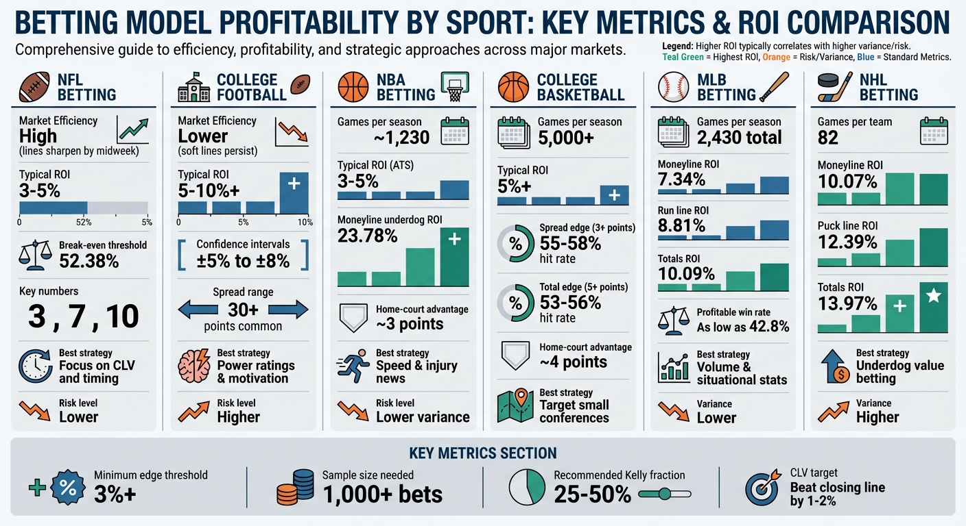
Betting Model Profitability Comparison Across Major Sports
Building profitable sports betting models #sportsbetting #mgcovers #sportsgambling
Football Betting Model Profitability (NFL and College)
Football betting models operate differently depending on whether you're focusing on the NFL or college football. The NFL's professional standards and salary cap create an environment where betting markets are highly efficient. Lines tend to sharpen quickly - often by midweek - as sharp bettors pounce on early odds. On the other hand, college football is a different beast. With vast talent gaps between powerhouse programs and smaller schools, along with a high volume of games and less media scrutiny, the market is less efficient. This means "soft" lines can linger, offering opportunities for models to uncover value.
The differences between these markets are significant. NFL totals usually fall within a narrow range, while college football totals can swing wildly, from 42 to 78 points. As one analyst aptly described:
"The NFL has structure. College football is fireworks in a wind tunnel."
- bcsguestwriter, Business of College Sports
This sets the stage for examining how betting strategies differ in these two arenas.
NFL Profitability by Bet Type
NFL betting models thrive on the league's predictability. Disciplined coaching and structured game scripts reduce randomness, allowing models to achieve high accuracy. However, this efficiency also means smaller edges. Totals (Over/Under) are often a strong focus for models, as they can incorporate metrics like Expected Points Added (EPA), success rates, and environmental factors such as wind and game pace. Wind, in particular, is a key factor for "Under" bets, as it disrupts passing and kicking - something models can quantify more effectively than the general public.
For spread betting, success often hinges on key numbers like 3 and 7, which are the most common victory margins in the NFL. Grabbing a line at +3.5 instead of +3.0 can make a significant difference over time. Moneyline bets, on the other hand, require precise probability estimates, as the bookmaker's vigorish (-110) creates a 52.38% break-even threshold. To stay profitable, models must consistently outperform this mark.
Timing is another critical factor in NFL betting. Early-week lines (Monday morning) tend to be softer, while sharp money tightens them by midweek. Late-week lines (Friday or Saturday) can reflect last-minute adjustments, such as quarterback injuries. A 2024 study by Jacob Conrad at Quinnipiac University analyzed 1,560 NFL games (2018–2023) and found that gradient boosting regression with forward selection outperformed sportsbook benchmarks, achieving a root mean squared error (RMSE) better than the standard 12.87 for point spreads.
These factors highlight the precision required to profit in the NFL, where the market's efficiency leaves little room for error. College football, however, offers a different kind of challenge - and opportunity.
College Football: Higher Variance, Better Opportunities
College football betting offers greater potential returns because of its inefficiencies. The disparity between top-ranked teams and unranked opponents creates edges that the NFL's parity doesn't allow. Add to this the diversity in coaching styles, emotional factors like rivalry games, and the influence of passionate fanbases, and you have a market ripe for mispricing.
The rise of Name, Image, and Likeness (NIL) compensation has made college football even more intriguing for betting models. For example, in the 2025–2026 season, University of Miami quarterback Carson Beck chose to stay in college for NIL deals instead of entering the NFL draft. This trend provides models with more data on key players, improving predictive capabilities.
That said, college football models come with higher uncertainty. Teams play only 12–15 games per season, and factors like roster turnover from the transfer portal and unpredictable coaching decisions add variability. Confidence intervals for college models often range from ±5% to ±8%, meaning any edge must exceed 8–10% to be worthwhile. As one analyst put it:
"College football betting is a different language. A different rhythm. And for those who understand the shift... the results often speak for themselves."
- bcsguestwriter, Business of College Sports
A practical strategy in college football is live betting on "flat" starts by heavy favorites. Books often overreact early, allowing savvy bettors to grab better spreads mid-game as the talent gap becomes evident. Additionally, college games frequently break traditional key numbers (3, 7, 10) due to missed extra points, two-point attempts, and blowouts, creating opportunities on alternative spreads.
These nuances make college football a fertile ground for models, despite the higher risks involved.
NFL vs. College Football: Side-by-Side Comparison
| Feature | NFL Betting Market | College Football Betting Market |
|---|---|---|
| Market Efficiency | High (Lines sharpen by midweek) | Lower (Soft lines persist longer) |
| Parity/Variance | High Parity (Slim margins) | High Variance (Massive talent gaps) |
| Typical Spreads | Tight (Rarely exceeds 17.5) | Wide (30+ point spreads common) |
| Totals Range | Narrow/Consistent | Wide (42 to 78+ points) |
| Key Numbers | Highly relevant (3, 7, 10) | Often broken by missed PATs/2-pt tries |
| Model Strategy | Focus on closing line value (CLV) | Focus on power ratings and motivation |
| Bankroll Management Risk | Lower (More predictable scripts) | Higher (Requires smaller unit sizes) |
| Best Timing | Early week (Monday) or late (Friday) for injuries | Thursday lines often still exploitable |
| Confidence Intervals | Tighter/More precise | Wider (±5% to ±8%) |
NFL betting demands precision and discipline to navigate its efficient markets. In contrast, college football's inefficiencies create opportunities for higher returns, but with greater uncertainty. Bettors should approach college football with smaller unit sizes to account for these risks, especially when betting on teams with limited data.
Basketball Betting Model Profitability (NBA and College)
Basketball betting models juggle the high volume of games with the challenge of sharp market efficiency. The NBA features about 1,230 games per season across 30 teams, while college basketball boasts over 5,000 games across more than 355 Division I programs [16, 19]. These differences create distinct betting environments. In the NBA, markets adjust quickly to news, making them highly efficient. On the other hand, college basketball markets often reveal gaps, as sportsbooks may not track every team with the same precision. Let’s break down how these conditions shape strategies for each.
The NBA’s efficiency makes it tough to find an edge. Tomas O'Connell notes, "The market, particularly if you're betting sides or totals for a game, is almost always close to what the 'true number' should be". Success often hinges on speed and timely information, especially around injuries. For example, learning that a key player like Giannis, Steph, or Jokic is out before sportsbooks adjust can lead to a 25% projected ROI. However, these windows close fast, and with standard -110 odds requiring a 52.4% win rate to break even [12, 13], there’s little room for error.
College basketball offers a different dynamic. Markets are less efficient early in the season, sharpening only around Weeks 8–11 when conference play begins. The talent gap between powerhouse programs and mid-major schools creates opportunities rarely seen in the NBA. Sportsbooks often struggle to set accurate lines for lesser-known teams in conferences like the Horizon League or Colonial Athletic Association, leaving room for well-designed models to succeed.
NBA Betting Models: Smaller Profit Margins
NBA betting models, while consistent, often yield smaller returns. For instance, one machine learning model using lagged variables achieved 63% raw accuracy and a steady 10% ROI over 1,500 bets. Another study analyzing 362 games with RAPTOR metrics showed a 3.53% ROI for betting against the spread (ATS) and a 23.78% ROI when targeting undervalued moneyline underdogs. Underdogs often provide better value in the NBA compared to point spreads.
Given the NBA’s 82-game season, bettors must automate tracking of injury reports and roster updates. Manual tracking increases the risk of missing critical information. Models that prioritize Closing Line Value (CLV) tend to perform better - if your predictions consistently differ from the closing line, it’s a sign your model may need improvement. Line shopping across sportsbooks is also crucial; even a half-point difference (e.g., -6.5 vs. -7) can significantly impact long-term profits.
One systematic NBA algorithm achieved an average ROI of 34.3% across all matchups, rising to 55.7% for games with spreads of 3 points or less. Tighter spreads often indicate more competitive matchups, which are generally easier to predict. However, the NBA’s low variance - teams average about 105 points per game with a 3-point home-court advantage - limits the size of potential edges.
While NBA models emphasize speed and efficiency, college models capitalize on volume and deeper statistical insights.
College Basketball: Better Returns Than NBA
College basketball models often deliver higher ROI potential compared to NBA models. For example, in January 2026, the ProPlotFits NCAA basketball model analyzed over 10,000 games from the 2023–24 and 2024–25 seasons. Its Gradient Boosting model for spreads achieved a Mean Absolute Error (MAE) of 8.7 points, while a Random Forest model for totals had an MAE of 10.9 points. Spread edges of 3+ points hit at a rate of 55–58%, and total edges of 5+ points hit at 53–56%. Additionally, their win probability models showed a historical backtest accuracy of 72%.
Profitability in college basketball relies on volume and variance. With over 5,000 games per season, models have more opportunities to uncover edges. The talent disparity between teams means dominant programs are more likely to cover large spreads - sometimes by 20 to 30 points - unlike the more balanced NBA. College teams score around 68 points per game with a 4-point home-court advantage. The 30-second shot clock (compared to the NBA’s 24 seconds) also reduces possession counts and overall scoring.
Timing plays a key role. Jason Scavone from Unabated explains, "There's not a lot of signal in early season CLV. It isn't until conference play starts up that even sharp bettors start getting a good enough feel for these teams". Early-season bets carry higher risk but also higher potential rewards. As the season progresses, metrics like CLV become more reliable, especially in smaller conferences where sportsbooks have less data [17, 19].
Both NBA and college models require over 1,000 bets to validate their predictive power, making scale essential.
NBA vs. College Basketball: Side-by-Side Comparison
| Feature | NBA Betting Models | College Basketball Models |
|---|---|---|
| Number of Teams | 30 | 355+ |
| Games Per Season | ~1,230 | 5,000+ |
| Market Efficiency | High (lines are very sharp) | Lower (especially in smaller conferences) |
| Typical ROI (ATS) | 3%–5% | 5%+ (often higher) |
| Moneyline Underdog ROI | 23.78% | Potentially higher in mid-majors |
| Spread Edge Threshold | Best at ±3 points or less | 3+ points hit at 55–58% |
| Total Edge Threshold | Varies | 5+ points hit at 53–56% |
| Primary Edge | Injury news and speed | Statistical modeling and volume |
| Home-Court Advantage | ~3 points | ~4 points |
| Average Points Per Game | ~105 | ~68 |
| Key Challenge | Overcoming the vig and rapid market adjustments | Fragmented data and high variance |
| Best Strategy | Focus on underdogs and tight spreads [13, 18] | Target small conferences and conference play [17, 19] |
| Sample Size Needed | 1,000+ bets | 1,000+ bets |
Both markets demand a large sample size to determine true predictive power. In the NBA, speed and automation are critical for leveraging brief opportunities. College basketball, however, rewards thorough research into lesser-known teams and conferences. While college betting models often yield higher ROIs in specific scenarios, the NBA provides more stable and predictable returns for disciplined bettors.
Baseball (MLB) and Hockey (NHL) Betting Model Profitability
When it comes to betting, MLB and NHL offer two very different landscapes. Both sports require strategies tailored to their unique dynamics, but the approaches for each couldn’t be more distinct. MLB’s long season of 162 games per team (a total of 2,430 games) provides a high-volume betting environment where small advantages can add up over time. On the other hand, the NHL’s shorter 82-game season means fewer opportunities, and its competitive balance brings more unpredictability. As Patrick Cwiklinski from Sportsbook Expert puts it:
"Baseball generally offers lower returns in the long run, but each team plays 162 games per season... this gives bettors a much more comfortable margin of error".
MLB: Consistency Through Volume
MLB betting thrives on volume. With so many games, bettors can quickly build a large enough sample size to make their strategies statistically meaningful. PJ Walsh from Sports Insights explains this advantage:
"The only difference between these two bettors is that a 2% edge in baseball offers exponentially more wagering opportunities than football and, in turn, a profit that's more than 9.5 times greater".
To break it down, a 2% ROI on 486 MLB bets can lead to a profit of +9.72 units, while the same edge over just 51 NFL bets would yield only +1.02 units.
MLB betting doesn’t require a sky-high win rate to be profitable. A model focusing on plus-money underdogs can succeed with a win rate as low as 42.8%. Situational factors like pitcher matchups, home/road splits, and recent performance are key to uncovering small but consistent edges. For example, betting on home underdogs with less than 30% of public moneyline bets has historically returned a 2.4% ROI. Among the most profitable teams, moneyline bets delivered a 7.34% ROI, run line bets returned 8.81%, and totals earned 10.09%.
Another factor working in MLB bettors’ favor is the summer season. Sportsbooks tend to be less accurate during this period, as other major sports are in their offseason.
While MLB’s consistency makes it appealing, NHL betting brings higher risks - and potentially higher rewards.
NHL: Managing Volatility for Bigger Payoffs
NHL betting comes with its own challenges, primarily due to the league’s parity. As Robert Ferringo from Doc's Sports points out:
"NHL teams are generally separated by razor thin margins, and you will absolutely go broke trying to bank on high moneyline favorites in hockey because no sport generates as many odd results".
This unpredictability makes underdog betting essential. The most profitable NHL teams have delivered impressive returns: moneyline bets averaged a 10.07% ROI, puck line bets returned 12.39%, and totals reached 13.97%.
Although the NHL’s shorter season means fewer opportunities than MLB, strategic betting can still yield strong results. First-period bets are one way to reduce the impact of late-game variability, while avoiding heavy favorites can help protect against frequent upsets. Unlike MLB, where lower variance allows for steadier returns, NHL bettors must be prepared for more dramatic swings. Success in hockey betting often hinges on spotting underdog value and accepting the sport’s inherent unpredictability.
MLB vs. NHL: A Quick Comparison
Here’s a side-by-side look at how MLB and NHL betting models differ:
| Feature | MLB Betting Models | NHL Betting Models |
|---|---|---|
| Games Per Season | 2,430 total (162 per team) | 82 per team |
| Market Efficiency | Less sharp during summer | – |
| Moneyline ROI | 7.34% | 10.07% |
| Spread/Puck Line ROI | 8.81% | 12.39% |
| Totals ROI | 10.09% | 13.97% |
| Variance | Lower (more forgiving margin for error) | Higher (frequent upsets due to parity) |
| Profitable Win Rate | As low as 42.8% (with plus-money underdogs) | Varies; underdog focus is key |
| Primary Edge | Volume and situational stats | Underdog value betting |
| Key Challenge | Small ROI requires high bet volume | High volatility and razor-thin margins |
| Best Strategy | Focus on home underdogs with minimal public bets | Avoid heavy favorites; focus on first-period bets |
Both sports demand a disciplined approach and careful bankroll management. While MLB rewards bettors who can consistently find small edges across its high volume of games, NHL offers more dramatic potential returns for those willing to navigate its volatility.
How to Maximize Betting Model Profitability
To get the most out of your betting model, you need a mix of smart bet sizing, sharp tools, and sport-specific tweaks. Let's break it down.
Bankroll Management for Each Sport
A solid betting strategy starts with bankroll management, and the Kelly Criterion is a key tool for this. The formula is simple: optimal bet size = (bp - q) / b, where b is net odds, p is win probability, and q is loss probability. But here's the catch: going full Kelly can be too aggressive. Instead, stick to fractional Kelly - betting 50% of the calculated amount for moderate risk or 25% for sports with more uncertainty.
Set a minimum edge threshold of at least 3% to account for errors and avoid losses from commissions. When placing multiple bets at once, reduce your Kelly fraction by the square root of the number of bets and keep your total exposure below 10% of your bankroll.
Another critical piece? Loss management rules. If your bankroll takes a 15% hit, cut your Kelly fraction in half. If you hit a 25% drawdown, pause new bets and analyze your model for issues. Regularly update your bankroll and adjust bet sizes as your capital changes.
Disciplined staking is just the start - pair it with advanced tools to find value.
Using WagerProof Tools and Data

WagerProof offers some powerful tools to help you identify value and refine your bets:
- The Edge Finder compares your model's predictions to market odds, highlighting outliers where multiple models agree on a pick. This consensus reduces the risk of relying on a single model's mistakes.
- The AI Game Simulator runs detailed simulations for each game, giving you precise win probabilities to plug into your Kelly calculations.
- WagerBot Chat keeps your bets current by cross-checking them with live updates, including injuries, weather, and lineup changes. For instance, a soccer model that broke even after 600 bets saw its ROI jump to 4.2% after adjusting for late-breaking lineup updates.
Additionally, the Model Aggregator combines over 50 statistical models, using z-scores to surface the most reliable picks.
"Expected value is the truth serum for your bets – it reveals whether you're making a savvy play or donating to the sportsbook's coffers".
Keep an eye on your Closing Line Value (CLV). A strong model should beat the closing line by 1% to 2% consistently. If you’re falling short, revisit your data inputs. And remember, you need at least 1,000 bets to draw meaningful conclusions about your model's success.
Adjusting for Sport-Specific Patterns
To improve profitability, tailor your model to the quirks of each sport:
- NFL: Passing efficiency is a major factor in winning. Over 75% of past Super Bowl champions outperformed their opponents by more than one yard per pass attempt. Use time-decay functions to adjust pregame spreads for live game variables like possession and score differences.
- MLB: Home underdogs with less than 30% of public moneyline bets have historically delivered a 2.4% ROI.
- NHL: Avoid heavy favorites and look at first-period bets to sidestep late-game volatility.
Break your bets into Core 4 segments - Home Favorites, Home Underdogs, Away Favorites, and Away Underdogs. Analyze ROI for each segment to pinpoint where your model performs best. Use metrics like ATS-WM (Against The Spread Win Margin) to determine if a team deserved to cover, helping you distinguish bad luck from deeper issues with your model.
Public bias can also create opportunities. For example, fading popular teams like the Cowboys - whose fan loyalty often skews betting lines - can yield profits. In high-variance sports like golf or horse racing, try the 80/20 strategy: allocate 80% of your stake on "place" bets and 20% on "win" bets. This approach balances risk and reward, especially since 80% of horse races are won by just 20% of jockeys and trainers. Focus your model on this elite group for better results.
Conclusion: What You Need to Know About Betting Model Profitability
Profitability in betting models varies widely by sport. For instance, college football and basketball often yield higher returns, while sports like MLB and NHL offer more consistent, albeit smaller, advantages. The crucial takeaway? Each sport demands a tailored mathematical approach. For example, Poisson distributions are ideal for predicting outcomes in low-scoring games like soccer or hockey, while logistic regression is better suited for binary outcomes such as NFL moneylines. This means there’s no one-size-fits-all strategy.
Your betting strategy should adapt to the unique characteristics of each sport. Market efficiency plays a big role - low-liquidity markets, such as NCAA props, often present greater opportunities compared to high-profile events like the NFL Super Bowl. Techniques like fractional Kelly sizing can help manage variance while maximizing long-term growth, making them invaluable for fine-tuning your approach.
Leveraging data-driven tools can significantly enhance your betting outcomes. These tools are capable of turning break-even models into consistent profit generators. Take, for example, a bettor’s soccer model in June 2025: by incorporating adjustments for real-time factors like lineup changes, the model improved ROI from 0% to 4.2% across 1,200 bets.
Success also hinges on understanding the market dynamics of your chosen sport. Tools like WagerProof's Edge Finder, AI Game Simulator, and WagerBot Chat provide real-time insights by comparing your predictions against professional data. These tools help identify outliers, consensus picks, and value bets. Additionally, tracking Closing Line Value (CLV) remains a cornerstone for spotting genuine edges. By consistently monitoring CLV alongside these tools, you can ensure your model stays sharp and responsive to evolving conditions.
Ultimately, disciplined adjustments, sport-specific strategies, and a commitment to using real-time data are essential for building and maintaining profitable betting models.
FAQs
Which sport is easiest to beat with a betting model?
Tennis is often seen as one of the simpler sports to analyze with a betting model. The game’s structure, featuring straightforward outcomes and fewer unpredictable factors, allows for more consistent and reliable predictions compared to many other sports.
How much CLV do I need for long-term profit?
To maintain long-term profitability, it’s essential to ensure your Customer Lifetime Value (CLV) remains consistently positive. A positive CLV means that, on average, your odds outperform the market's closing odds, which are considered a reflection of true value and predictive accuracy. Over time, sustaining positive CLV across a large number of bets becomes a stronger indicator of future Return on Investment (ROI) than focusing on short-term wins or losses.
How do I set my bet size with fractional Kelly?
To determine your bet size using fractional Kelly, start by calculating the full Kelly fraction with this formula:
[ f^* = \frac{bp - q}{b} ]
Here’s what each variable represents:
- b: Net odds (calculated as decimal odds minus 1)
- p: Your estimated probability of winning
- q: The probability of losing (1 - p)
Once you have the full Kelly fraction, multiply it by your total bankroll. To manage risk and minimize fluctuations, bet only a portion of this amount - like 25% or 50% of the calculated value. This approach helps maintain a balance between potential growth and risk control.
Related Blog Posts
Ready to bet smarter?
WagerProof uses real data and advanced analytics to help you make informed betting decisions. Get access to professional-grade predictions for NFL, College Football, and more.
Get Started Free